Smooth Manifolds
Charts, tangent spaces, and the language of calculus on curved spaces
Overview & Motivation
The Earth is round, but every map you have ever used is flat. A navigator’s chart takes a patch of the globe — say, the North Atlantic — and lays it out on a plane where you can draw straight lines, measure distances with a ruler, and do Euclidean geometry. A different chart covers the South Pacific. Where the charts overlap, a transition map tells you how to convert coordinates from one chart to the other. The key insight: as long as these transition maps are smooth, you can do calculus on the sphere by doing calculus on the flat charts and translating back.
This is exactly what a smooth manifold is: a space that is locally Euclidean — every point has a neighborhood that looks like a patch of — with a collection of charts whose transitions are smooth. The definition captures an enormous family of spaces: spheres, tori, the configuration space of a robot arm, the space of probability distributions in statistics, and the parameter spaces of neural networks.
Why should an ML practitioner care? Three reasons.
-
Data lives on manifolds. High-dimensional datasets often concentrate near lower-dimensional curved surfaces. Manifold learning algorithms (Isomap, LLE, t-SNE, UMAP) assume this structure explicitly. Understanding the tangent space at a point is the first step toward understanding local geometry, and tangent-space PCA (PCA & Low-Rank Approximation) is the workhorse of local dimensionality reduction.
-
Optimization happens on manifolds. Constraints force parameters onto curved spaces — orthogonal matrices form the manifold , positive-definite matrices form an open cone, and probability simplices are manifolds with boundary. Riemannian optimization generalizes gradient descent to these settings, and the theory starts here.
-
Information geometry is manifold geometry. The space of parametric probability distributions is a smooth manifold, and the Fisher information metric turns it into a Riemannian manifold. The natural gradient, KL divergence, and the geometry of exponential families all live in this framework — but the foundations require smooth manifolds, tangent spaces, and the differential.
What We Cover
- Topological Manifolds — the definition: locally Euclidean, Hausdorff, second-countable.
- Charts and Atlases — coordinate charts, transition maps, and smooth compatibility.
- Smooth Manifolds — smooth atlases, maximal atlases, and the smooth structure.
- A Gallery of Smooth Manifolds — spheres, tori, projective spaces, and matrix Lie groups.
- Smooth Maps & Diffeomorphisms — smoothness via charts, the inverse function theorem on manifolds.
- Tangent Vectors & Tangent Spaces — derivations, the tangent space as a vector space, coordinate bases.
- The Differential (Pushforward) — the derivative of maps between manifolds, the chain rule, immersions and submersions.
- Partitions of Unity — gluing local constructions into global ones.
- Computational Notes — stereographic projection code, symbolic tangent vectors, numerical tangent space estimation.
- The Whitney Embedding Theorem & Connections — every manifold embeds in Euclidean space; connections to the rest of formalML.
The prerequisites are the Spectral Theorem (for the linear algebra of tangent spaces) and Simplicial Complexes (for the topological intuition). We assume familiarity with multivariable calculus and basic point-set topology (open sets, continuity, homeomorphisms).
Topological Manifolds
Before we can talk about smooth structure, we need the underlying topological space to behave well. A topological manifold is a space that locally looks like Euclidean space and has enough topological regularity to support analysis.
Definition 1 (Topological Manifold).
A topological manifold of dimension is a topological space that satisfies three conditions:
- Hausdorff: For any two distinct points , there exist disjoint open sets and .
- Second-countable: has a countable basis for its topology.
- Locally Euclidean of dimension : Every point has an open neighborhood that is homeomorphic to an open subset of .
The Hausdorff condition rules out pathological spaces like the “line with two origins,” where two points cannot be separated by open sets. Second-countability ensures that the topology is not too large — it guarantees the existence of partitions of unity (which we will need later) and makes the space paracompact.
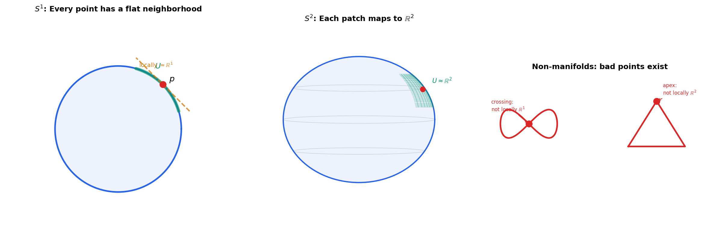
The heart of the definition is condition (3): local Euclideanness. Around every point , we can find a neighborhood that “looks like” a piece of . The homeomorphism is a coordinate system — it assigns real numbers to each point near .
Examples.
- is an -dimensional topological manifold: take and the identity map.
- The circle is a 1-manifold: every point has a small arc around it that is homeomorphic to an open interval in .
- The sphere is a 2-manifold: every point has a small cap homeomorphic to a disk in .
- Any open subset of is an -manifold (open subsets of manifolds are manifolds).
Non-examples.
- A figure-eight (two circles sharing a point) is not a manifold: at the crossing point, no neighborhood is homeomorphic to an interval — it looks like a cross, not a line segment.
- A cone with its apex is not a 2-manifold at the apex: the apex has no neighborhood homeomorphic to an open disk.
Charts and Atlases
A topological manifold tells us that coordinate systems exist locally. We now formalize what a coordinate system is and what happens where two coordinate systems overlap.
Definition 2 (Chart (Coordinate Chart)).
A chart on a topological manifold is a pair where is an open set and is a homeomorphism onto an open subset of . The set is the coordinate neighborhood (or chart domain), and is the coordinate map. For a point , the components are the local coordinates of .
A single chart rarely covers the entire manifold. The sphere , for instance, cannot be covered by a single chart — there is no homeomorphism from to an open subset of (a topological obstruction: is compact, and open subsets of are not). We need multiple charts, and we need them to be compatible where they overlap.
Definition 3 (Atlas).
An atlas on is a collection of charts such that the chart domains cover :
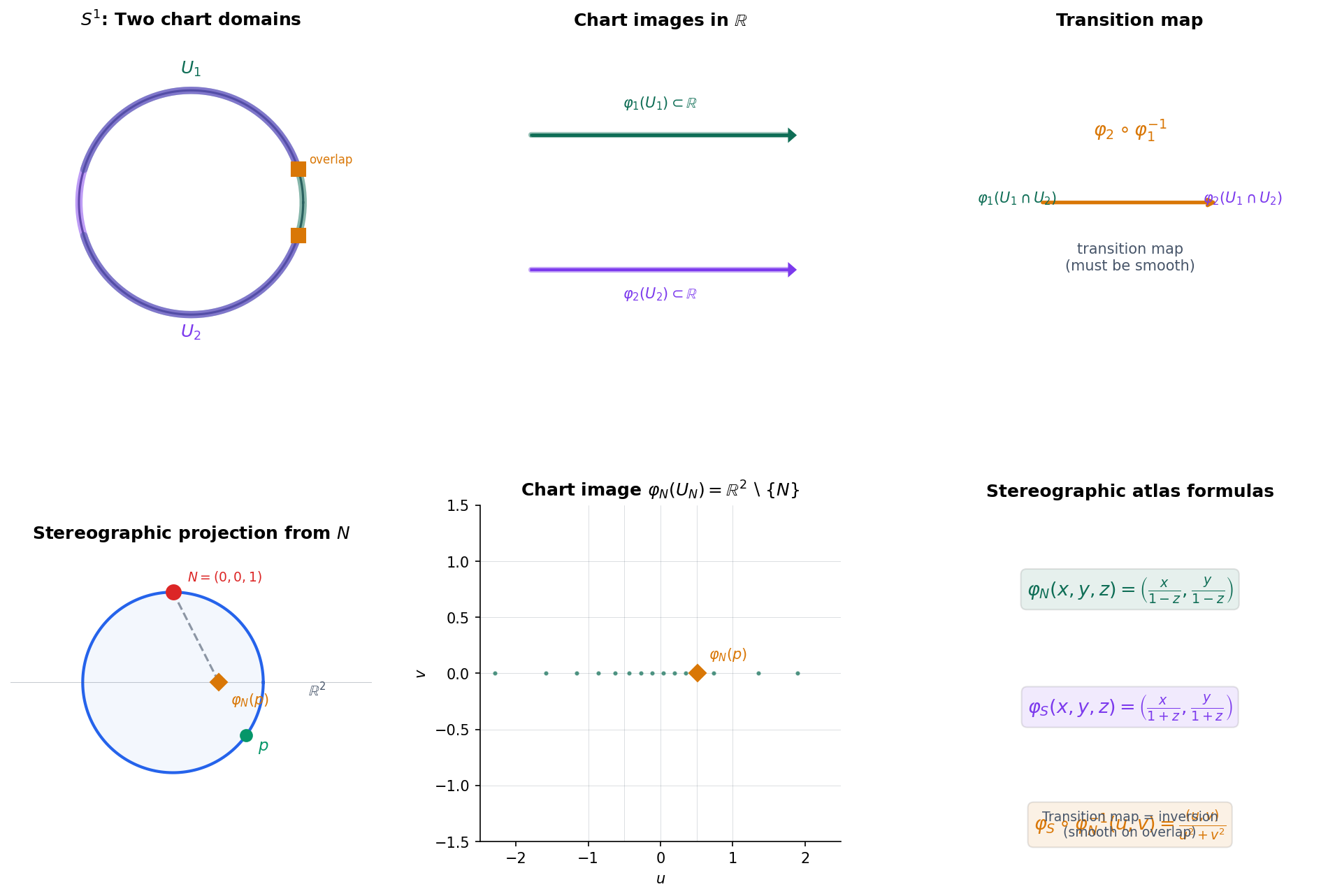
Where two charts and overlap — that is, when — we can ask: how do the two coordinate systems relate? The answer is the transition map.
The transition map from chart to chart is the composite
This is a map between open subsets of — familiar territory where we know exactly what “smooth” means. The smoothness of the transition maps is what will let us do calculus on .
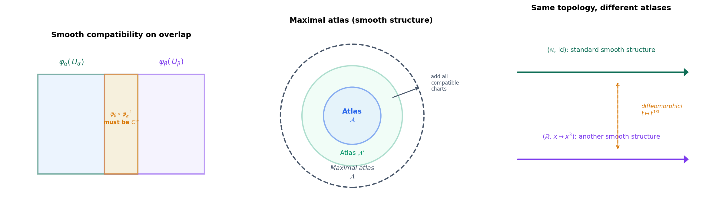
Definition 4 (Smoothly Compatible Charts).
Two charts and on are smoothly compatible if either , or the transition map
is a diffeomorphism (smooth with smooth inverse) between open subsets of .
Worked example: Stereographic projection on . The stereographic atlas for the sphere uses two charts:
- North pole chart : the domain is everything except the north pole . The map projects from the north pole onto the equatorial plane:
- South pole chart : the domain is everything except the south pole . The map projects from the south pole:
The overlap is — the sphere minus both poles. The transition map acts on by:
This is the inversion map — smooth (and in fact real-analytic) on , with itself as its own inverse. The two charts are smoothly compatible, so is a smooth atlas on .
Smooth Manifolds
We now have all the ingredients to define the central object.
Definition 5 (Smooth Atlas).
An atlas on is a smooth atlas if every pair of charts in is smoothly compatible — that is, all transition maps are diffeomorphisms.
A smooth atlas specifies how to do calculus on : a function is “smooth” if, for every chart in the atlas, the composite is a smooth function on an open subset of . But there is a subtlety: different smooth atlases might define the same notion of “smooth function.” Two smooth atlases and are compatible if their union is also a smooth atlas. Compatible atlases define the same calculus, so we want to identify them.
The cleanest way to do this is to take the maximal atlas: the collection of all charts that are smoothly compatible with a given atlas.
Definition 6 (Smooth Manifold).
A smooth manifold is a pair where is a topological manifold and is a maximal smooth atlas — a smooth atlas that is not properly contained in any larger smooth atlas. The maximal atlas is called the smooth structure on .
In practice, we never write down the maximal atlas explicitly. We specify a smooth atlas , and the maximal atlas is the unique one containing : it consists of all charts that are smoothly compatible with every chart in . Two smooth atlases determine the same smooth structure if and only if their union is still a smooth atlas.
When do two atlases give different smooth structures? Consider with two atlases:
- — the identity chart.
- where .
The transition map is smooth, but its inverse is not smooth at (the derivative blows up). So and are not compatible — they define different smooth structures on . However, the map given by is a diffeomorphism, so the two smooth structures are diffeomorphic (the same up to relabeling). This is a general phenomenon for , but not for all manifolds — exotic smooth structures on and show that distinct non-diffeomorphic smooth structures can exist on the same topological manifold.
A Gallery of Smooth Manifolds
The definition might seem abstract, but smooth manifolds are everywhere. Here is a tour of the most important examples, each illustrating a different way that smooth structures arise.
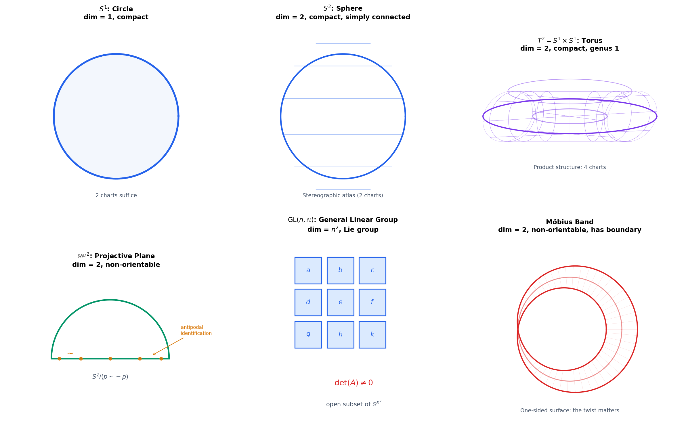
The -sphere . The unit sphere is a smooth -manifold. The stereographic atlas (two charts, projecting from opposite poles) provides a smooth atlas with two charts. For , this is the circle; for , the ordinary sphere. The sphere is compact (closed and bounded in ) and simply connected for (every loop can be contracted to a point).
The torus . The 2-torus is the product of two circles. As a smooth manifold, its smooth structure is the product structure: if and are charts on , then is a chart on . The torus is compact with fundamental group (genus 1). It can be parametrized by
for , where are the major and minor radii.
Real projective space . The real projective space is the set of lines through the origin in , or equivalently the quotient (identifying antipodal points). It is a smooth -manifold with standard charts. For , is the projective plane — non-orientable (it contains a Mobius band) and cannot be embedded in without self-intersections.
Matrix Lie groups. The general linear group is an open subset of , hence a smooth manifold of dimension . It is a Lie group: a smooth manifold that is also a group, with smooth multiplication and inversion.
The orthogonal group is a smooth manifold of dimension (the orthogonality condition imposes independent constraints on entries). The Spectral Theorem tells us that orthogonal matrices have eigenvalues on the unit circle — the spectral structure constrains the geometry of .
The special orthogonal group is the connected component of the identity in , and represents pure rotations. For , is diffeomorphic to — every rotation is determined by an axis (a line through the origin) and an angle.
Smooth Maps & Diffeomorphisms
With smooth manifolds defined, the next question is: what does it mean for a map between manifolds to be smooth? Since we only know how to differentiate functions on , we route through the charts.
Definition 7 (Smooth Map).
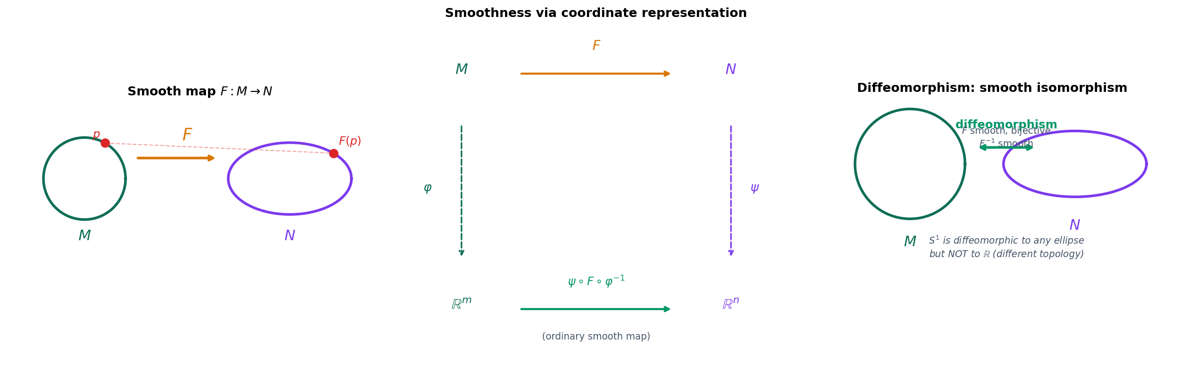
Let and be smooth manifolds. A continuous map is smooth if for every point , there exist charts around in and around in such that the coordinate representation
is a smooth map between open subsets of Euclidean space.
The coordinate representation is the map “as seen in the charts.” We check smoothness in where we know what that means. But we need this to be independent of which charts we choose — otherwise the definition would be chart-dependent and hence meaningless.
Proposition 1 (Smoothness Is Chart-Independent).
If is smooth with respect to one pair of charts around and , then it is smooth with respect to every pair of compatible charts.
Proof.
Let and be charts around in , and let and be charts around in . Suppose is smooth. Then
The outer factors and are transition maps — smooth by the atlas compatibility condition. The middle factor is smooth by assumption. A composition of smooth maps is smooth, so is smooth.
∎This is precisely why we required the transition maps to be smooth: it ensures that the notion of “smooth map” does not depend on the choice of charts.
Definition 8 (Diffeomorphism).
A smooth map is a diffeomorphism if it is bijective and its inverse is also smooth. If a diffeomorphism exists between and , we write and say they are diffeomorphic.
Diffeomorphisms are the isomorphisms in the category of smooth manifolds. Two diffeomorphic manifolds are “the same” as smooth objects — they have the same dimension, the same smooth functions, and the same differential-geometric invariants.
Theorem 1 (Inverse Function Theorem on Manifolds).
Let be a smooth map between smooth manifolds of the same dimension. If the differential is an isomorphism (i.e., the Jacobian of the coordinate representation is invertible), then there exists an open neighborhood of such that is a diffeomorphism onto an open subset of .
This is the manifold version of the classical inverse function theorem from multivariable calculus. It says that a smooth map is locally invertible wherever its derivative is invertible — the same statement, now on curved spaces.
Tangent Vectors & Tangent Spaces
We have smooth manifolds and smooth maps. The next step is the derivative — but the derivative of what? On , the derivative of a function at a point is a linear map that tells us how changes in each direction. On a manifold, we need to define “directions” without relying on an ambient Euclidean space.
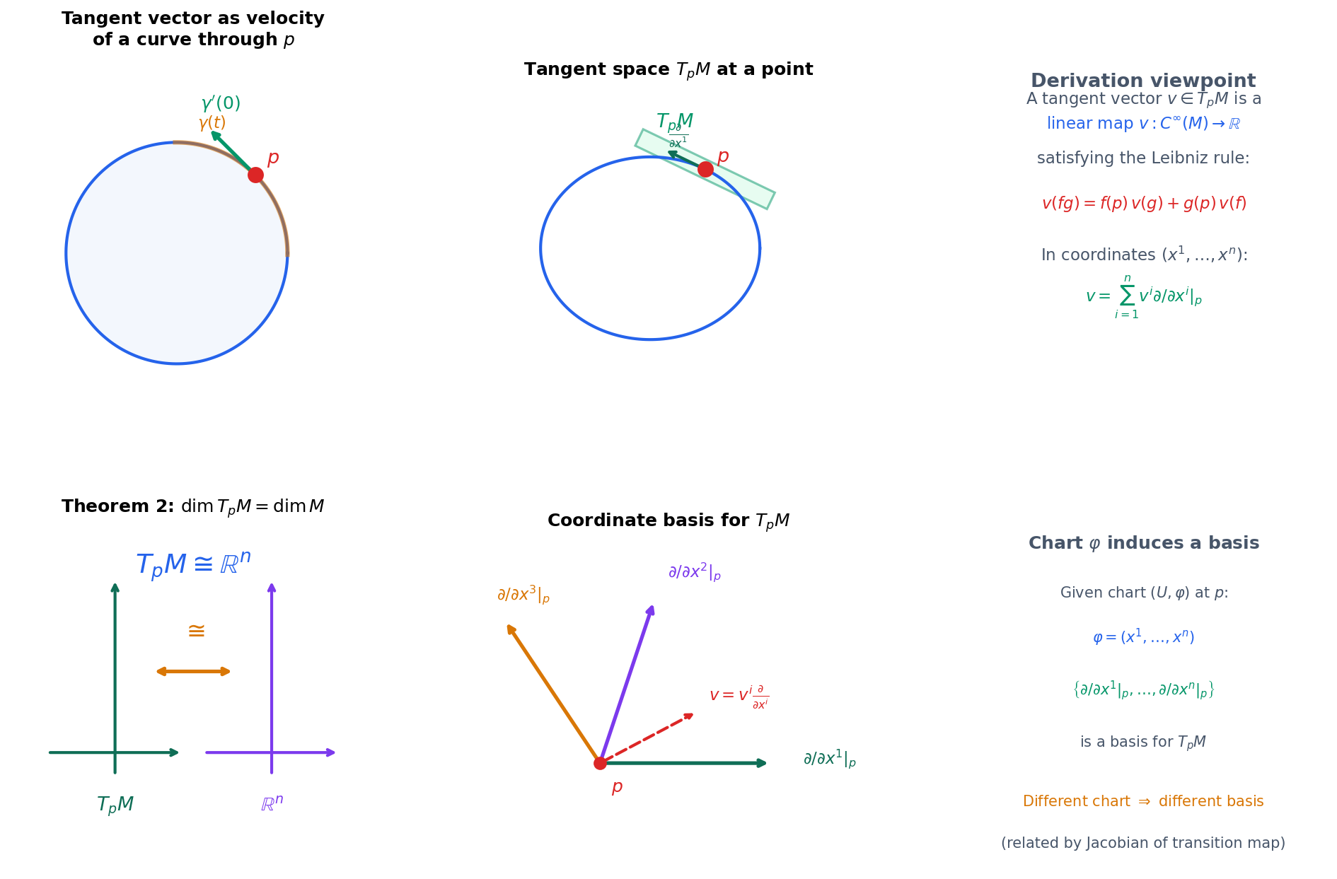
The geometric picture is clear: a tangent vector at a point on a surface is the velocity vector of a curve passing through . If is a smooth curve with , then should be a tangent vector at . But “velocity” requires a notion of derivative, which we are trying to define. The resolution is elegant: we define tangent vectors algebraically, as operators on smooth functions.
Definition 9 (Tangent Vector (Derivation)).
Let be a smooth manifold and . A tangent vector at is a linear map that satisfies the Leibniz rule (product rule):
where denotes the algebra of smooth real-valued functions on .
A tangent vector “eats” a smooth function and returns a number — the directional derivative of the function in the direction of the vector. The Leibniz rule is the product rule, the defining property of differentiation.
The connection to curves. If is a smooth curve with , then the operator
is a derivation at . Every derivation arises this way — there is a one-to-one correspondence between tangent vectors as derivations and equivalence classes of curves through (where two curves are equivalent if they have the same velocity in any chart).
Definition 10 (Tangent Space).
The tangent space to at , denoted , is the set of all tangent vectors (derivations) at . With pointwise addition and scalar multiplication of linear maps, is a real vector space.
Theorem 2 (Dimension of the Tangent Space).
If is a smooth manifold of dimension , then is an -dimensional real vector space for every . In particular, as vector spaces.
Proof.
Let be a chart around with coordinate functions . Define the coordinate basis vectors by
where are the standard coordinates on .
We claim that is a basis for .
Linear independence. Apply to the coordinate function :
If , then applying this to gives for all .
Spanning. Let be any derivation. Set . For any , write in local coordinates as . By Taylor’s theorem in with the Leibniz rule, one shows that
so . Thus .
∎The coordinate basis depends on the chart, but the tangent space itself does not. A different chart gives a different basis related by the Jacobian of the transition map — the same change-of-basis story from linear algebra.
The tangent space is where the linear algebra of the Spectral Theorem comes alive on manifolds. Once we equip each tangent space with an inner product (a Riemannian metric), the tangent space becomes an inner product space, and its self-adjoint operators have spectral decompositions. The eigenvalues of the curvature operator at each point encode the principal curvatures — but that is the story of Riemannian Geometry.
The Differential (Pushforward)
We have tangent spaces at every point. Now we need the manifold version of the derivative: a linear map between tangent spaces that tells us how a smooth map transforms infinitesimal displacements.
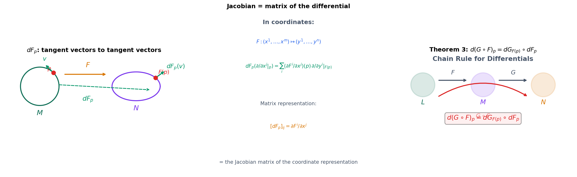
Definition 11 (The Differential (Pushforward)).
Let be a smooth map and . The differential of at is the linear map defined by
The differential is also called the pushforward and sometimes denoted or .
In words: to push forward a tangent vector at along , we define a new tangent vector at that acts on test functions by first pulling back to (composing with ) and then applying .
In coordinates. Let be a chart around and a chart around , with coordinate functions on and on . The coordinate representation of is , with components . Then
The matrix is the Jacobian matrix of at in these coordinates. The differential is the coordinate-free version of the Jacobian.
The Singular Value Decomposition of the Jacobian matrix reveals how stretches and rotates infinitesimal neighborhoods: the singular values are the principal stretches, and the left and right singular vectors give the principal directions of stretching in the target and source tangent spaces.
Theorem 3 (Chain Rule for Differentials).
Let and be smooth maps between smooth manifolds. Then for all ,
In coordinates, this is matrix multiplication of Jacobians: .
Proof.
Let and . Then
The first equality is the definition of . The third equality is the definition of . The fourth is the definition of . Since this holds for all , we have for all .
∎The chain rule on manifolds says that the derivative of a composition is the composition of derivatives — exactly the same statement as in multivariable calculus, now liberated from coordinates.
Immersions and submersions. A smooth map is an immersion at if is injective (the Jacobian has full column rank). It is a submersion at if is surjective (the Jacobian has full row rank). If is an isomorphism (bijective), then the Inverse Function Theorem (Theorem 1) guarantees that is a local diffeomorphism near .
These rank conditions classify the local behavior of smooth maps: immersions locally look like linear inclusions (with ), and submersions locally look like linear projections (with ).
Partitions of Unity
One of the deepest differences between smooth manifolds and general topological spaces is the existence of partitions of unity: families of smooth functions that sum to 1 and allow us to glue local constructions into global ones.
Definition 12 (Partition of Unity).
Let be an open cover of a smooth manifold . A smooth partition of unity subordinate to the cover is a collection of smooth functions such that:
- Support condition: for each (each is zero outside ).
- Local finiteness: Every point has a neighborhood that intersects only finitely many of the sets .
- Partition condition: for all .
Theorem 4 (Existence of Smooth Partitions of Unity).
Every open cover of a smooth manifold admits a smooth partition of unity subordinate to it.
Proof (Proof sketch).
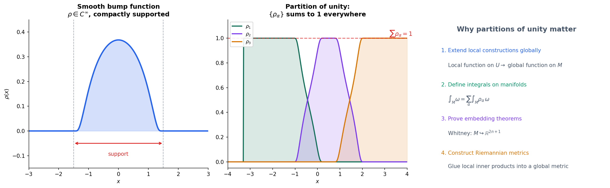
The proof has three ingredients. First, the existence of smooth bump functions: for any point and open neighborhood , there exists a smooth function that equals 1 near and vanishes outside . (In , the standard construction uses mollifiers; the charts carry this to .)
Second, paracompactness: every open cover of has a locally finite refinement. This follows from second-countability (condition 2 of the topological manifold definition). We refine to a locally finite cover, construct bump functions for each element of the refinement, and group them by which they refine.
Third, normalization: given bump functions with and everywhere (which follows from the covering property), set . The sum in the denominator is locally finite, hence smooth, and the resulting satisfies all three conditions.
∎Why partitions of unity matter. They are the technical engine behind almost every “local-to-global” argument in differential geometry:
-
Extending local to global. If you have a smooth function defined on an open subset of , a partition of unity lets you extend it to all of (possibly changing it outside ).
-
Defining integrals on manifolds. To integrate a function on , cover with charts, multiply by partition-of-unity functions to localize, integrate each piece in , and sum: .
-
Constructing Riemannian metrics. Any smooth manifold admits a Riemannian metric. Proof: on each chart, use the standard Euclidean inner product; then use a partition of unity to average them into a global metric. (This is how the existence of metrics on all smooth manifolds is proved — it’s a direct application of Theorem 4.)
-
The Whitney embedding theorem. The proof that every smooth manifold embeds in Euclidean space uses partitions of unity to build a global embedding from local coordinate maps.
Computational Notes
The abstract definitions become concrete — and computationally useful — when we implement them. Here we work through key computations that connect the theory to code.
Stereographic Projection
The stereographic atlas on is the running example throughout this topic. Here it is in Python:
import numpy as np

def stereo_north(x, y, z):
    """Stereographic projection from the north pole: S^2 \ {N} -> R^2."""
    return x / (1 - z), y / (1 - z)

def stereo_south(x, y, z):
    """Stereographic projection from the south pole: S^2 \ {S} -> R^2."""
    return x / (1 + z), y / (1 + z)

def inv_stereo_north(u, v):
    """Inverse stereographic projection (north pole chart)."""
    d = u**2 + v**2
    return 2*u / (1 + d), 2*v / (1 + d), (d - 1) / (1 + d)

def transition_NS(u, v):
    """Transition map: phi_S ∘ phi_N^{-1}(u, v) = (u, v) / (u^2 + v^2)."""
    r2 = u**2 + v**2
    return u / r2, v / r2
We can verify the transition map: applying transition_NS to the north-pole coordinates of a point should give the south-pole coordinates of the same point.
# Point on S^2: (x, y, z) = (1/sqrt(2), 0, 1/sqrt(2))
x, y, z = 1/np.sqrt(2), 0, 1/np.sqrt(2)
u_N, v_N = stereo_north(x, y, z)    # North pole chart coordinates
u_S, v_S = stereo_south(x, y, z)    # South pole chart coordinates
u_T, v_T = transition_NS(u_N, v_N)  # Via transition map

print(f"Direct south pole coords: ({u_S:.6f}, {v_S:.6f})")
print(f"Via transition map:       ({u_T:.6f}, {v_T:.6f})")
# Both give the same result — the transition map works.
Symbolic Tangent Vectors with SymPy
The tangent space at a point is spanned by the coordinate basis vectors . In the stereographic chart, these are:
import sympy as sp

u, v = sp.symbols('u v')

# Inverse stereographic projection (north pole chart)
d = u**2 + v**2
x_expr = 2*u / (1 + d)
y_expr = 2*v / (1 + d)
z_expr = (d - 1) / (1 + d)

# Tangent vectors: partial derivatives of the parametrization
du_tangent = sp.Matrix([sp.diff(x_expr, u), sp.diff(y_expr, u), sp.diff(z_expr, u)])
dv_tangent = sp.Matrix([sp.diff(x_expr, v), sp.diff(y_expr, v), sp.diff(z_expr, v)])

print("∂/∂u =", sp.simplify(du_tangent).T)
print("∂/∂v =", sp.simplify(dv_tangent).T)
Jacobian of Stereographic Projection
The differential of the stereographic projection has a Jacobian that reveals conformal stretching:
# Jacobian of the transition map (inversion)
u_out = u / (u**2 + v**2)
v_out = v / (u**2 + v**2)

J = sp.Matrix([
    [sp.diff(u_out, u), sp.diff(u_out, v)],
    [sp.diff(v_out, u), sp.diff(v_out, v)]
])

print("Jacobian of transition map:")
sp.pprint(sp.simplify(J))
# Result: (1/(u^2+v^2)^2) * [[v^2-u^2, -2uv], [-2uv, u^2-v^2]]
# This is a conformal map: J = (1/r^2) * rotation
Numerical Tangent Space Estimation
Given a point cloud sampled near a manifold, we can estimate the tangent space at a point using PCA. The key insight: near a point on an -manifold embedded in , the local point cloud is approximately flat in the tangent directions and thin in the normal directions. The top principal components span (approximately) .
from sklearn.decomposition import PCA

def estimate_tangent_space(points, p, k=50, n_components=2):
    """Estimate the tangent space at p from a local neighborhood."""
    # Find k nearest neighbors of p
    dists = np.linalg.norm(points - p, axis=1)
    neighbors = points[np.argsort(dists)[:k]]

    # Local PCA: top n_components directions approximate T_pM
    pca = PCA(n_components=n_components)
    pca.fit(neighbors - p)  # Center at p
    return pca.components_  # Rows are tangent basis vectors

# Example: points on S^2, estimate tangent plane at the north pole
theta = np.random.uniform(0, 0.3, 500)  # Small polar angle (near north pole)
phi = np.random.uniform(0, 2*np.pi, 500)
points = np.column_stack([
    np.sin(theta)*np.cos(phi),
    np.sin(theta)*np.sin(phi),
    np.cos(theta)
])

tangent_basis = estimate_tangent_space(points, p=np.array([0, 0, 1]))
print("Estimated tangent basis:")
print(tangent_basis)
# Should be approximately [[1, 0, 0], [0, 1, 0]] — the xy-plane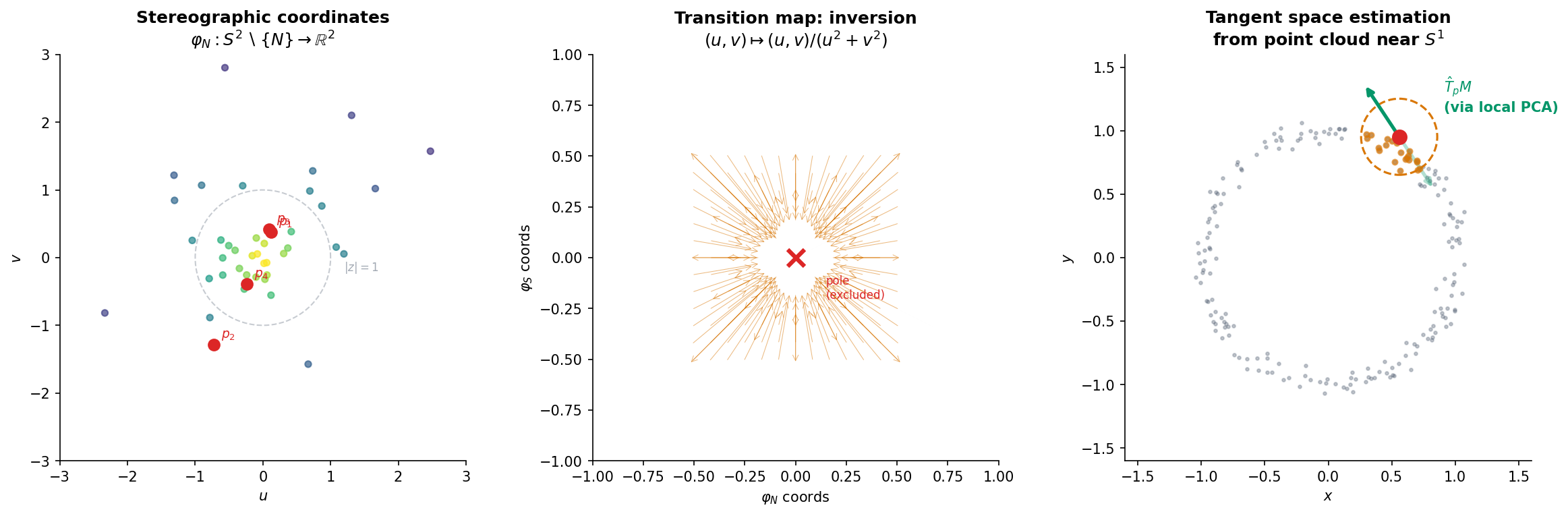
The Whitney Embedding Theorem & Connections
We close with a theorem that bridges the intrinsic and extrinsic viewpoints, and then connect the theory to the rest of the formalML curriculum.
The Whitney Embedding Theorem
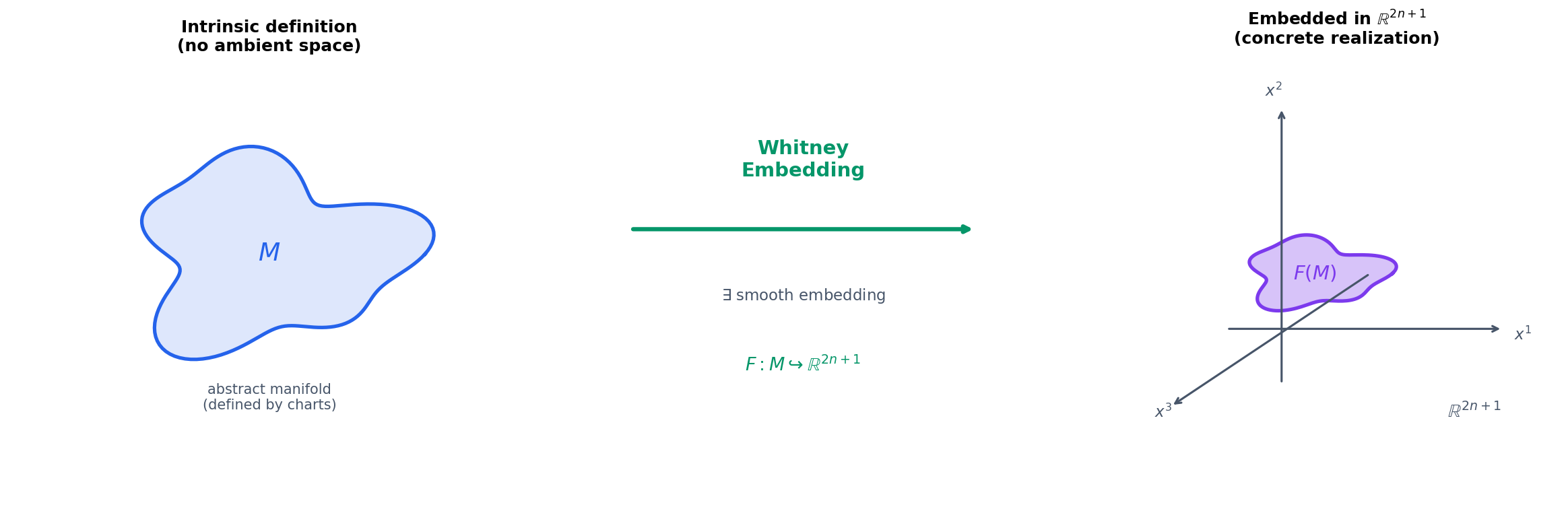
Throughout this topic, we have defined smooth manifolds intrinsically — via charts and transition maps, with no reference to an ambient Euclidean space. But many of the examples we drew intuition from — the sphere in , the torus in — are subsets of Euclidean space. Is this always possible? Can every abstract smooth manifold be realized as a “surface” in some ?
Theorem 5 (Whitney Embedding Theorem).
Every smooth -manifold admits a smooth embedding into .
More precisely, if is a smooth manifold of dimension , then there exists an injective smooth immersion that is a homeomorphism onto its image — a smooth embedding.
The dimension bound is sharp in the sense that there exist -manifolds that cannot be embedded in (though many specific manifolds embed in much lower dimensions). The proof uses partitions of unity (Theorem 4) to assemble local coordinate embeddings into a global one, and a transversality argument to ensure injectivity in dimension .
Geometric meaning. No matter how abstractly a manifold is defined — even if it is constructed as a quotient, a fiber bundle, or an inverse image of a regular value — it can always be concretely realized as a subset of Euclidean space. The intrinsic viewpoint (charts and transition maps) and the extrinsic viewpoint (submanifolds of ) are equivalent.
Examples of the dimension bound:
- (): embeds in — well below the guarantee.
- (): embeds in — below the guarantee.
- (): embeds in — again below the guarantee.
- The Klein bottle (): cannot embed in (non-orientable surfaces self-intersect in ), but embeds in — still below .
Where This Goes Next
Smooth manifolds are the foundation for three planned topics in the Differential Geometry track:
-
Riemannian Geometry — equip each tangent space with an inner product (a metric tensor). The Spectral Theorem then applies at every point: the eigenvalues of the metric encode how the manifold stretches in different directions. Riemannian metrics make it possible to measure lengths, angles, and volumes on curved spaces.
-
Geodesics & Curvature — the differential (§7) tells us how maps curve, and the Riemannian metric (from the next topic) tells us how the manifold itself curves. Geodesics are the “straight lines” of curved spaces, and curvature quantifies how the manifold deviates from flatness.
-
Information Geometry & Fisher Metric — a parametric family of probability distributions is a smooth manifold (the parameter space ). The Fisher information matrix is a Riemannian metric on this manifold. The natural gradient, KL divergence, and the geometry of exponential families all live in this framework — the direct connection between smooth manifolds and machine learning.
Connections to Other Tracks
The theory in this topic connects to several topics across other tracks on formalML:
-
The Spectral Theorem: The tangent space is a real vector space. Once equipped with a Riemannian metric, the curvature operator on is a self-adjoint linear map whose eigenvalues (principal curvatures) are computed via the Spectral Theorem.
-
Simplicial Complexes: Smooth manifolds can be triangulated — decomposed into simplicial complexes. This connects the combinatorial topology of homology (Betti numbers, Euler characteristic) with the differential topology of tangent spaces and smooth maps.
-
Singular Value Decomposition: The differential is a linear map between finite-dimensional vector spaces. Its SVD decomposes the map into principal stretches (singular values) and principal directions (singular vectors), revealing exactly how distorts infinitesimal geometry.
-
PCA & Low-Rank Approximation: Tangent-space PCA estimates the tangent space from data sampled near a manifold. This is the foundation of manifold learning algorithms that use local linear approximations to discover low-dimensional structure in high-dimensional data.
Connections
- The tangent space at each point of an n-manifold is an n-dimensional real vector space. Inner products on tangent spaces (Riemannian metrics) produce symmetric bilinear forms whose matrices in local coordinates are symmetric and can be diagonalized via the Spectral Theorem; similarly, the self-adjoint shape operator has eigenvalues that are the principal curvatures. spectral-theorem
- Simplicial complexes provide a combinatorial model of topological spaces. Smooth manifolds can be triangulated into simplicial complexes, connecting the combinatorial topology of homology with the differential topology of tangent spaces and smooth maps. simplicial-complexes
- The differential (pushforward) of a smooth map between manifolds is a linear map between tangent spaces. Its SVD reveals how the map stretches and rotates infinitesimal neighborhoods — the singular values are the principal stretches. svd
- PCA on data sampled from a manifold estimates the tangent space at a point. Tangent-space PCA is the foundation of local dimensionality reduction methods like local PCA and manifold learning algorithms. pca-low-rank
References & Further Reading
- book Introduction to Smooth Manifolds — Lee (2013) Chapters 1-5: The primary graduate reference for smooth manifolds, charts, tangent spaces, and smooth maps
- book An Introduction to Manifolds — Tu (2011) Chapters 1-8: Accessible undergraduate-to-graduate treatment with careful exposition of tangent vectors as derivations
- book Differential Geometry: Connections, Curvature, and Characteristic Classes — Tu (2017) Chapter 1: Smooth manifolds review, connecting to vector bundles and curvature
- book Foundations of Differential Geometry, Vol. I — Kobayashi & Nomizu (1963) Chapter I: Differentiable manifolds — the classical reference for the foundations
- paper The Easy Part of the Whitney Embedding Theorem — Shastri (2011) Clean proof of the weak Whitney embedding theorem (2n+1 dimensions) used in exposition
- paper Manifold Learning: What, How, and Why — Izenman (2012) Connects smooth manifold theory to modern dimensionality reduction and manifold learning in data science