Singular Value Decomposition
From rectangular matrices to the geometry of linear maps — the most useful factorization in data science
Overview & Motivation
The Spectral Theorem told us that every symmetric matrix decomposes into orthogonal eigenvectors and real eigenvalues. That’s powerful — but it only works for square, symmetric matrices. Most matrices we meet in practice are neither.
A data matrix with observations in features is . A term-document matrix in NLP is . An image is . None of these are square. None are symmetric. The Spectral Theorem says nothing about them directly.
The Singular Value Decomposition fills this gap. Every matrix — any shape, any rank — has an SVD:
where and are orthogonal and is diagonal with non-negative entries. The diagonal entries are the singular values, and they measure how much the matrix stretches space in each direction. The columns of are the input directions, and the columns of are the output directions.
This decomposition is the single most useful factorization in applied mathematics. It powers:
- PCA: the principal components of a centered data matrix are exactly the right singular vectors of .
- Low-rank approximation: the truncated SVD is the best rank- approximation to (Eckart–Young theorem).
- The pseudoinverse: solves least-squares problems.
- Image compression: keeping only the top singular values compresses an image with provably minimal error.
- Latent Semantic Analysis: SVD on a term-document matrix discovers hidden topic dimensions.
- Condition numbers: measures numerical sensitivity.
What We Cover
- From the Spectral Theorem to the SVD — why and are the key.
- The SVD: Statement and Proof — existence, the four forms, the outer product expansion.
- Geometric Interpretation — the SVD as rotate–stretch–rotate; the four fundamental subspaces; the pseudoinverse.
- Low-Rank Approximation — the Eckart–Young–Mirsky theorem and truncated SVD.
- Computing the SVD in Practice —
numpy.linalg.svd, theVtpitfall, randomized SVD. - Image Compression — truncated SVD on grayscale images.
- Latent Semantic Analysis — SVD on term-document matrices for concept discovery.
- The SVD–PCA Connection — right singular vectors are principal components.
From the Spectral Theorem to the SVD
The Key Insight: and
Let be any matrix (not necessarily square or symmetric). Consider the two products:
- — symmetric and PSD, since .
- — symmetric and PSD, since .
By the Spectral Theorem, both and have orthogonal eigendecompositions with real non-negative eigenvalues. The SVD arises from the observation that these two eigendecompositions are intimately linked.
Shared Eigenvalues
Proposition 1 (Shared eigenvalues of $A^T A$ and $A A^T$).
and have the same nonzero eigenvalues.
Proof.
Suppose with . Set . Then:
So is an eigenvector of with the same eigenvalue . The converse direction is symmetric: if with , then satisfies .
∎Singular Values
Definition 1 (Singular values and singular vectors).
The singular values of are the square roots of the nonzero eigenvalues of (equivalently, of ):
ordered as where . The corresponding eigenvectors of are the right singular vectors , and the eigenvectors of are the left singular vectors . They satisfy .
The SVD: Statement and Proof
Theorem 1 (Singular Value Decomposition).
Let with . Then there exist:
- An orthogonal matrix (columns are left singular vectors),
- An orthogonal matrix (columns are right singular vectors),
- A diagonal matrix with entries on the diagonal and zeros elsewhere,
such that .
Proof.
Via the Spectral Theorem applied to .
Step 1. is symmetric and PSD (we showed this above). By the Spectral Theorem, there exists an orthogonal matrix and non-negative eigenvalues such that . Exactly of these eigenvalues are positive (since ). Set for .
Step 2. For , define . We verify that is orthonormal:
For : . For : .
Step 3. Extend to an orthonormal basis of (Gram–Schmidt on any complementary vectors). Set .
Step 4. We have for and for (since when ). In matrix form, this gives , hence .
∎Forms of the SVD
Definition 2 (Forms of the SVD).
| Form | Size | |||
|---|---|---|---|---|
| Full | All singular vectors | |||
| Thin | singular vectors | |||
| Compact | Only singular vectors | |||
| Truncated | Only the top singular vectors |
The outer product form expands the compact SVD as a sum of rank-1 matrices:
Each term is a rank-1 matrix, weighted by the singular value . This is the representation that makes the Eckart–Young theorem transparent.
import numpy as np

A = np.array([
    [1, 2, 0],
    [0, 1, 3],
    [2, 0, 1],
    [1, 1, 1]
], dtype=float)

# Compute the thin SVD
U, sigma, Vt = np.linalg.svd(A, full_matrices=False)
print(f"U shape: {U.shape}")   # (4, 3) — thin
print(f"Σ: {sigma.round(4)}")  # [3.8826, 2.2465, 1.6966]
print(f"Vt shape: {Vt.shape}") # (3, 3)

# Verify: A = U @ diag(sigma) @ Vt
A_reconstructed = U @ np.diag(sigma) @ Vt
print(f"||A - UΣVᵀ||_F = {np.linalg.norm(A - A_reconstructed):.2e}")

# Outer product form: A = sum sigma_i * u_i * v_i^T
A_outer = sum(sigma[i] * np.outer(U[:, i], Vt[i, :])
              for i in range(len(sigma)))
print(f"||A - Σ σᵢ uᵢvᵢᵀ||_F = {np.linalg.norm(A - A_outer):.2e}")
Geometric Interpretation
Rotate–Stretch–Rotate
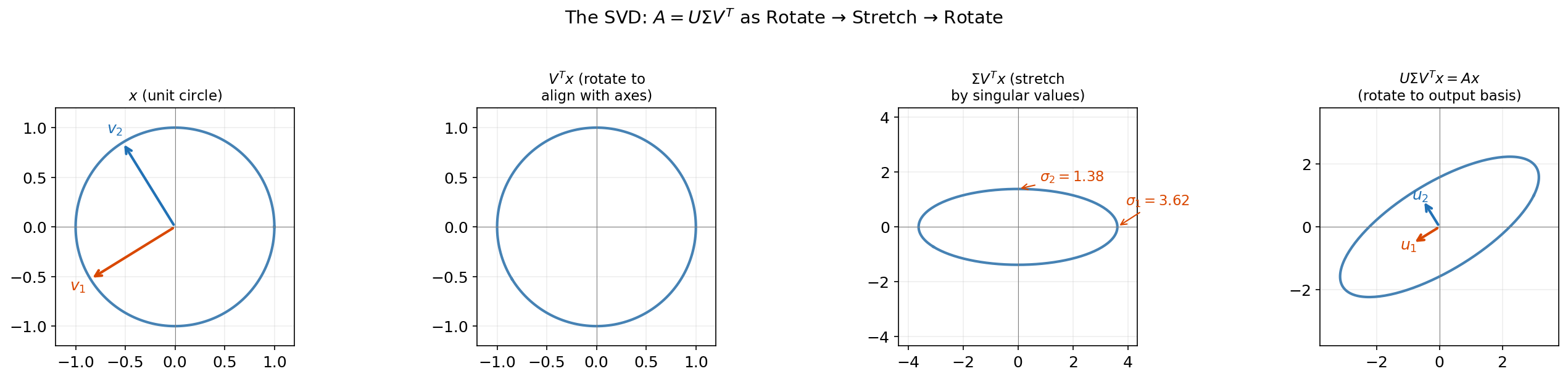
The SVD tells us that every linear map is a rotation, followed by an axis-aligned stretch, followed by another rotation. This is the geometric content of :
- rotates the input space to align the right singular vectors with the coordinate axes.
- stretches each axis by the corresponding singular value .
- rotates the result to align with the left singular vectors in the output space.
Drag the sliders below to explore this decomposition for any 2×2 matrix. Watch how the unit circle transforms through each step. Toggle “Make symmetric” to see how the SVD reduces to the Spectral Theorem when .
The Four Fundamental Subspaces
Definition 3 (The four fundamental subspaces).
The SVD reveals all four fundamental subspaces of with rank :
| Subspace | Symbol | Basis from SVD | Dimension |
|---|---|---|---|
| Column space (range) | |||
| Left null space | |||
| Row space | |||
| Null space |
These four subspaces satisfy and .
The Pseudoinverse
Definition 4 (Moore–Penrose pseudoinverse).
For with rank , the pseudoinverse is:
where is obtained by transposing and inverting the nonzero diagonal entries. satisfies (projection onto the row space) and (projection onto the column space). For the least-squares problem , the minimum-norm solution is .
Low-Rank Approximation
The Truncated SVD
Given the outer product form , we can approximate by keeping only the first terms:
This is the rank- truncated SVD. It throws away the smallest singular values and their associated directions. The question is: how good is this approximation?
The answer is: optimal.
The Eckart–Young–Mirsky Theorem
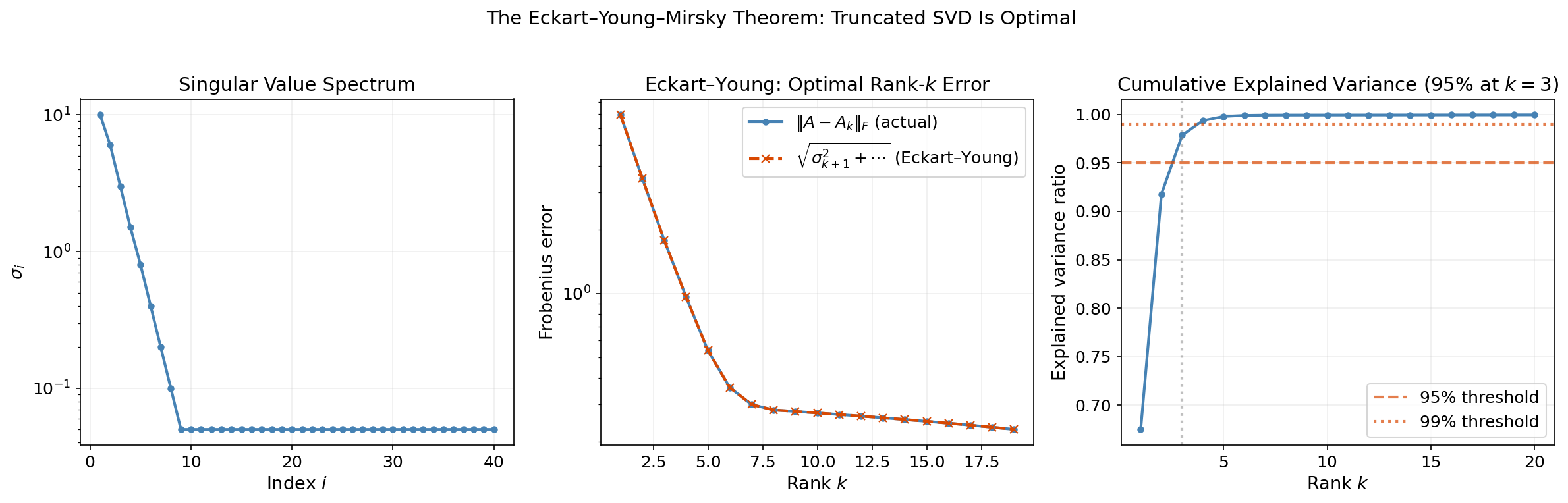
Theorem 2 (Eckart–Young–Mirsky Theorem).
Let with singular values . For any , the rank- truncated SVD is the best rank- approximation to in both the Frobenius and spectral norms:
Proof.
Frobenius norm. We use three facts: (1) the Frobenius norm is unitarily invariant, ; (2) the Frobenius norm of a diagonal matrix is the root-sum-of-squares of its entries; (3) has the SVD , so .
Now suppose has rank . Then has dimension . The subspace has dimension . Since , these subspaces must intersect — there exists a unit vector .
Write with . Then , so:
Since , this shows achieves the minimum in spectral norm. For the Frobenius norm bound, apply the same dimension argument iteratively to show that .
∎Explained Variance
Definition 5 (Explained variance ratio).
The fraction of total “energy” retained by the rank- approximation is:
This ratio tells us how much of the matrix’s structure we capture with components.
Drag the rank slider below to see how the Eckart–Young theorem plays out on a 16×12 matrix. Watch the difference heatmap shrink as you increase rank, and track the Frobenius error dropping.
Computing the SVD in Practice
NumPy and SciPy
Two main functions for computing the SVD in Python:
import numpy as np
from scipy.sparse.linalg import svds

# Dense SVD (full or thin)
U, sigma, Vt = np.linalg.svd(A, full_matrices=False)  # thin SVD

# CAUTION: numpy returns Vt (V-transpose), NOT V.
# This is the single most common SVD bug in practice.
# To reconstruct: A ≈ U @ np.diag(sigma) @ Vt
# NOT: A ≈ U @ np.diag(sigma) @ V

# Sparse SVD (for large matrices, top k components only)
U_k, sigma_k, Vt_k = svds(A_sparse, k=50)
Remark.
The Vt pitfall. numpy.linalg.svd returns , not . Nearly every SVD tutorial, homework solution, and production codebase has been bitten by this at least once. The variable name in numpy is literally Vt — use it. If you see code that does U @ np.diag(sigma) @ V, that’s a bug.
The Golub–Kahan Algorithm (Sketch)
The standard algorithm for computing the SVD in practice (used internally by LAPACK, which numpy calls) works in two phases:
- Bidiagonalization: Reduce to upper bidiagonal form using Householder reflections. This costs for .
- Diagonalization: Apply the implicit QR algorithm to (iteratively chasing off-diagonal entries to zero). Each iteration costs , and convergence is typically cubic.
The total cost is for the thin SVD of an matrix with .
Randomized SVD
For very large matrices where we only need the top singular values, the randomized SVD of Halko, Martinsson, and Tropp (2011) is dramatically faster:
def randomized_svd(A, k, p=10):
    """
    Randomized SVD: compute rank-k approximation of A.

    Parameters:
        A: (m, n) matrix
        k: target rank
        p: oversampling parameter (default 10)

    Returns:
        U_k, sigma_k, Vt_k: truncated SVD components
    """
    m, n = A.shape
    l = k + p  # oversampled rank

    # Step 1: Random projection to find approximate range of A
    Omega = np.random.randn(n, l)       # random test matrix
    Y = A @ Omega                        # project A onto random subspace
    Q, _ = np.linalg.qr(Y)              # orthonormal basis for range(Y)

    # Step 2: Form the small matrix B = Q^T A (l × n)
    B = Q.T @ A

    # Step 3: Compute exact SVD of the small matrix B
    U_tilde, sigma, Vt = np.linalg.svd(B, full_matrices=False)

    # Step 4: Recover U = Q @ U_tilde
    U = Q @ U_tilde

    # Truncate to rank k
    return U[:, :k], sigma[:k], Vt[:k, :]
The key insight: is an matrix whose columns approximately span the column space of . The QR factorization gives us an orthonormal basis , and then we only need to SVD the small matrix . Total cost: instead of .
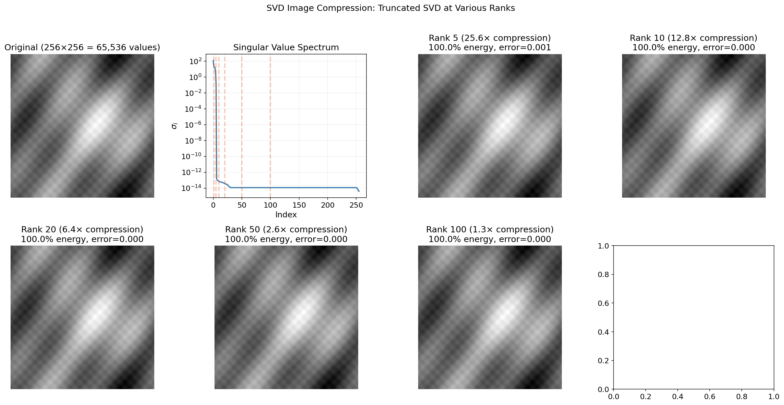
Application: Image Compression
A grayscale image is a matrix of pixel intensities. The SVD decomposes it into rank-1 “image layers,” each capturing structure at a different scale. The leading singular values correspond to large-scale gradients and shapes; the trailing ones encode fine textures and noise.
The rank- truncated SVD stores only numbers instead of — a compression ratio of . For a image with , that’s a 5× compression with the Eckart–Young guarantee of optimality.
Drag the rank slider to watch the image sharpen as you add more singular values:
# SVD image compression
from PIL import Image
import numpy as np

img = np.array(Image.open('photo.png').convert('L'), dtype=float)
U, sigma, Vt = np.linalg.svd(img, full_matrices=False)

# Reconstruct at rank k
k = 50
img_k = U[:, :k] @ np.diag(sigma[:k]) @ Vt[:k, :]

# Statistics
storage_original = img.shape[0] * img.shape[1]
storage_compressed = k * (img.shape[0] + img.shape[1] + 1)
energy = np.sum(sigma[:k]**2) / np.sum(sigma**2)

print(f"Rank-{k}: {storage_compressed/storage_original:.1%} of original")
print(f"Energy retained: {energy:.1%}")
print(f"Frobenius error: {np.sqrt(np.sum(sigma[k:]**2)):.2f}")
Application: Latent Semantic Analysis
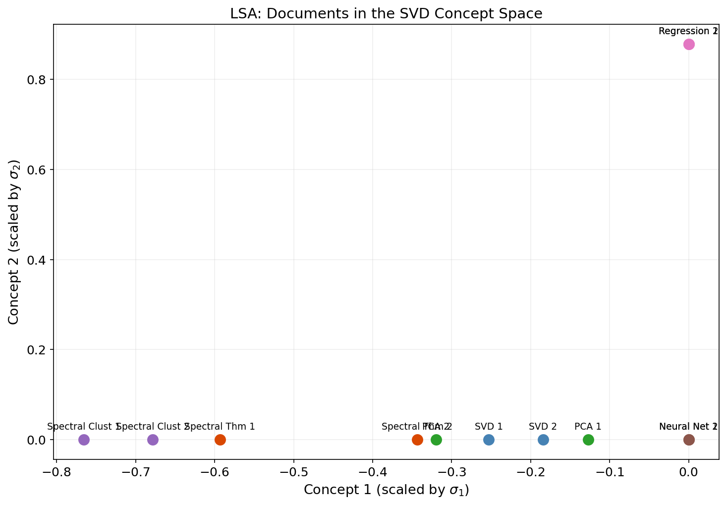
In natural language processing, a term-document matrix has rows indexed by vocabulary terms and columns indexed by documents, with entries measuring word frequency (often TF-IDF weighted). This matrix is large, sparse, and noisy. The truncated SVD discovers latent semantic dimensions — hidden topic structure that explains word co-occurrence patterns.
The idea: if “car” and “automobile” never appear in the same document but both co-occur with “engine,” “highway,” and “driving,” the SVD discovers that they belong to the same latent dimension. Documents that use different words but discuss the same topic will have similar representations in the SVD coordinate system.
The procedure is simple:
- Build the term-document matrix (often TF-IDF weighted).
- Compute the rank- truncated SVD: .
- The rows of give -dimensional document embeddings.
- The rows of give -dimensional term embeddings.
- Cosine similarity in the reduced space measures semantic similarity.
from sklearn.feature_extraction.text import TfidfVectorizer
from scipy.sparse.linalg import svds

# Build TF-IDF matrix
corpus = [
    "the cat sat on the mat",
    "the dog chased the cat",
    "the cat and dog played",
    "linear algebra is beautiful",
    "matrices and vectors are fundamental",
    "eigenvalues describe matrix behavior",
]
vectorizer = TfidfVectorizer()
A = vectorizer.fit_transform(corpus)

# Truncated SVD for LSA
k = 2
U, sigma, Vt = svds(A.T, k=k)  # transpose: docs as rows

# svds returns singular values in ascending order — reverse to descending
idx = np.argsort(sigma)[::-1]
U, sigma, Vt = U[:, idx], sigma[idx], Vt[idx, :]

# Document embeddings in concept space
doc_embeddings = Vt.T * sigma  # (n_docs, k)

# Cosine similarity between documents
from sklearn.metrics.pairwise import cosine_similarity
sim = cosine_similarity(doc_embeddings)
print("Document similarity (in SVD concept space):")
print(sim.round(3))
This is Latent Semantic Analysis (Deerwester et al., 1990) — the original word embedding technique, and still one of the clearest examples of why the SVD matters for machine learning.
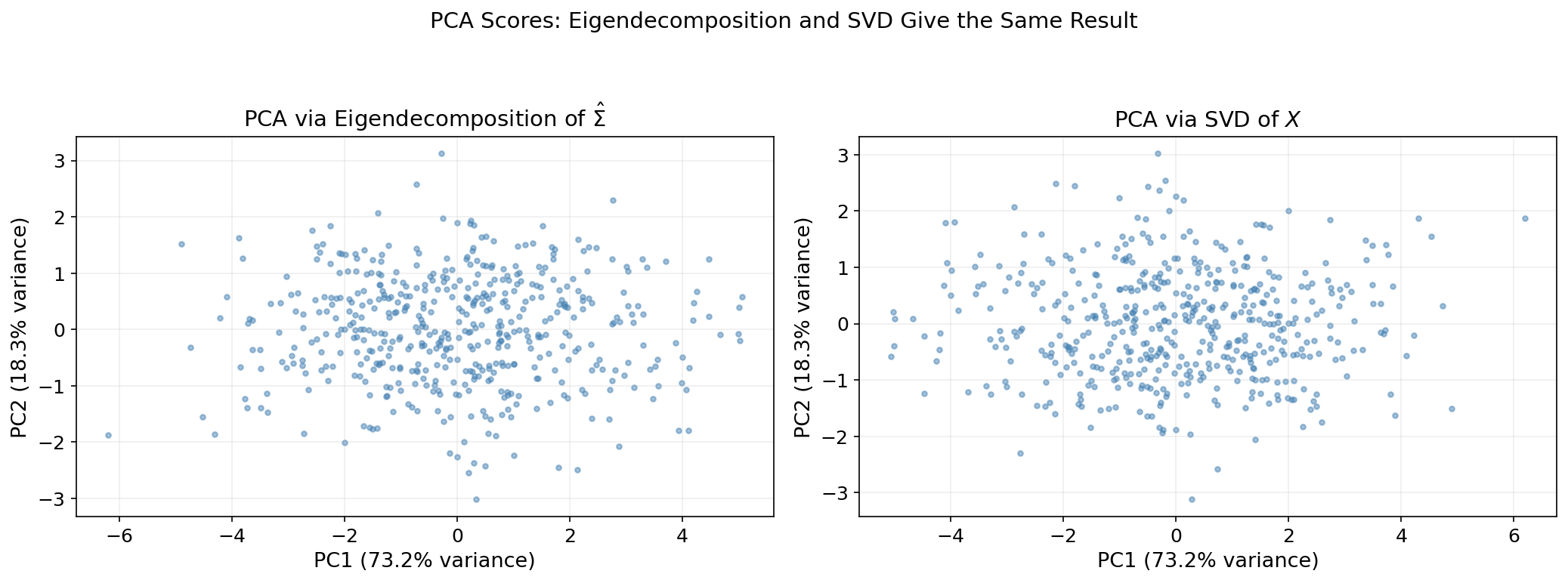
The SVD–PCA Connection
PCA computes the directions of maximum variance in a centered data matrix (rows = observations). The standard approach is to eigendecompose the sample covariance matrix . But the SVD provides a numerically superior alternative.
Let be the thin SVD. Then:
This is exactly the spectral decomposition of . We read off:
- Principal components: the columns of (right singular vectors of ).
- Eigenvalues of : .
- Projected data: (the principal component scores).
The SVD approach is numerically superior because it avoids forming — which squares the condition number. If , then , and eigendecomposition of may lose 8 digits of precision. The SVD of itself keeps full precision.
# PCA via SVD vs. covariance eigendecomposition
X = np.random.randn(100, 5)
X -= X.mean(axis=0)  # center the data

# Method 1: eigendecomposition of covariance matrix
Sigma_hat = (X.T @ X) / (X.shape[0] - 1)
eigenvalues, Q = np.linalg.eigh(Sigma_hat)
eigenvalues = eigenvalues[::-1]  # descending
Q = Q[:, ::-1]

# Method 2: SVD of data matrix
U, sigma, Vt = np.linalg.svd(X, full_matrices=False)
pca_eigenvalues = sigma**2 / (X.shape[0] - 1)

# They match
print(f"Eigenvalues (eigh):  {eigenvalues.round(6)}")
print(f"Eigenvalues (SVD):   {pca_eigenvalues.round(6)}")
print(f"Max difference:      {np.max(np.abs(eigenvalues - pca_eigenvalues)):.2e}")

# Principal components match (up to sign)
print(f"\nPC directions match: {np.allclose(np.abs(Q), np.abs(Vt.T))}")
The full PCA development, including the scree plot heuristic and the connection to the Eckart–Young theorem for optimal projection, appears on the PCA & Low-Rank Approximation topic page.
Connections & Further Reading
The SVD sits at the center of the Linear Algebra track, connecting backward to the Spectral Theorem and forward to PCA and tensor methods. It also has deep connections to the Topology & TDA track.
| Topic | Connection |
|---|---|
| The Spectral Theorem | The SVD proof relies on the Spectral Theorem applied to . For symmetric , the SVD reduces to the spectral decomposition — singular values are absolute eigenvalues, and (up to sign). |
| PCA & Low-Rank Approximation | PCA is the SVD of the centered data matrix. Principal components are right singular vectors. The Eckart–Young theorem makes the truncated SVD the optimal low-rank projection. |
| Tensor Decompositions | The CP decomposition generalizes the SVD outer product form to tensors: . HOSVD extends the SVD to multilinear algebra. |
| Persistent Homology | The boundary matrices in a simplicial complex have an SVD. The rank of determines Betti numbers, and the singular values quantify topological feature strength. |
| Sheaf Theory | The coboundary map in the Sheaf Laplacian has an SVD whose singular values are the square roots of the Sheaf Laplacian’s eigenvalues — connecting SVD to sheaf cohomology. |
| The Mapper Algorithm | Mapper often uses SVD-based dimensionality reduction (PCA or LSA) as the filter function that maps high-dimensional data to a lower-dimensional lens space. |
The Linear Algebra Track
Spectral Theorem
    ├── Singular Value Decomposition (this topic)
    │       └── PCA & Low-Rank Approximation
    └── Tensor Decompositions
Connections
- the SVD proof relies on the Spectral Theorem applied to AᵀA; for symmetric A, the SVD reduces to the spectral decomposition spectral-theorem
- PCA is the SVD of the centered data matrix; the Eckart–Young theorem makes the truncated SVD the optimal low-rank projection pca-low-rank
- the CP decomposition generalizes the SVD outer product form to tensors; HOSVD extends the SVD to multilinear algebra tensor-decompositions
- SVD of boundary matrices reveals Betti numbers; singular values quantify topological feature strength persistent-homology
- the coboundary map δ₀ in the Sheaf Laplacian has an SVD whose singular values are the square roots of the Sheaf Laplacian eigenvalues sheaf-theory
- Mapper often uses SVD-based dimensionality reduction (PCA, LSA) as the filter function mapper-algorithm
References & Further Reading
- book Introduction to Linear Algebra — Strang (2016) Chapter 7: SVD development and four fundamental subspaces
- book Matrix Analysis — Horn & Johnson (2013) Rigorous SVD existence and uniqueness proofs
- book Numerical Linear Algebra — Trefethen & Bau (1997) Golub–Kahan bidiagonalization and computational SVD
- book Matrix Computations — Golub & Van Loan (2013) The definitive reference for SVD algorithms
- paper Finding structure with randomness: Probabilistic algorithms for constructing approximate matrix decompositions — Halko, Martinsson & Tropp (2011) Randomized SVD algorithm
- paper The approximation of one matrix by another of lower rank — Eckart & Young (1936) Original Eckart–Young low-rank approximation theorem
- paper Indexing by Latent Semantic Analysis — Deerwester, Dumais, Furnas, Landauer & Harshman (1990) Original LSA paper
- paper Toward a spectral theory of cellular sheaves — Hansen & Ghrist (2019) Sheaf Laplacian spectral theory — cross-track connection