Sheaf Theory
From local data to global consistency — the algebraic geometry of gluing
Overview & Motivation
Across the six topics in this track, a single idea has appeared over and over: local information assembled into global structure. Simplicial complexes glue simplices into spaces. Persistent homology tracks how local connectivity merges into global topology across scales. The Mapper algorithm patches local clusters into a global nerve. Barcodes and bottleneck distance give us stable metrics on these global summaries.
Sheaf theory is the mathematical framework that makes this local-to-global pattern precise.
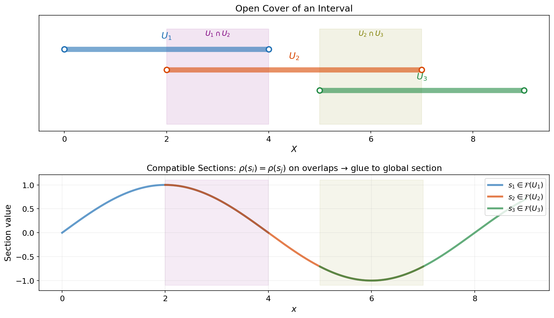
A sheaf assigns data to the open sets of a topological space (or the cells of a complex) and specifies how local pieces restrict to overlaps and glue into global sections. When data is consistent across overlaps, it glues into a global section. When it isn’t, the obstruction to gluing is measured by sheaf cohomology — a sequence of vector spaces that generalize the Betti numbers of ordinary homology.
Here is a concrete motivating example. Suppose three temperature sensors are placed around a room. Each sensor reports a local measurement, and on every pair of nearby sensors we have a calibration function that relates their readings. If all calibrations are consistent — sensor A agrees with sensor B, B agrees with C, and A agrees with C through the chain — the local readings glue into a single global temperature field. If they don’t agree, the size of the inconsistency is a meaningful quantity. Sheaf theory gives us the exact algebraic machinery to define, measure, and minimize this inconsistency.
This capstone topic covers the full sheaf-theoretic toolkit:
- Presheaves and Sheaves on topological spaces — the classical definitions.
- Cellular Sheaves on Graphs — where the theory becomes computational.
- Sheaf Cohomology — (global consistency) and (obstruction to gluing).
- The Sheaf Laplacian — a spectral operator that generalizes the graph Laplacian.
- Cosheaves and Duality — the dual perspective.
- Applications — sensor networks, opinion dynamics, multi-modal fusion.
Presheaves and Sheaves
The Idea: Data Organized by Open Sets
The starting point is deceptively simple: we want to assign data to regions of a space, in a way that is compatible when regions overlap.
Let be a topological space with open sets .
Definition 1 (Presheaf).
A presheaf on assigns:
- To each open set , a set (or vector space, group, etc.) , called the sections over .
- To each inclusion , a restriction map .
These satisfy two axioms:
- Identity: for every open set .
- Composition: If , then .
In the language of category theory, a presheaf is a contravariant functor from the category of open sets (with inclusions as morphisms) to the category of sets (or vector spaces). The “contravariant” means that restriction maps go in the opposite direction of inclusions: a smaller open set receives data from a larger one.
The Sheaf Condition
A presheaf becomes a sheaf when local data can be glued uniquely.
Definition 2 (Sheaf).
A presheaf is a sheaf if for every open cover of an open set :
-
Locality (Separation): If satisfy for all , then . (A global section is determined by its local restrictions.)
-
Gluing: If sections are compatible — meaning for all — then there exists a section with for all .
Example 1.
Continuous functions as a sheaf. Let and define , the set of continuous real-valued functions on . The restriction maps are literal restriction of functions: . This is a sheaf because:
- Locality: If two continuous functions agree on every open set in a cover, they are the same function.
- Gluing: If we have continuous functions on overlapping open sets that agree on overlaps, they glue into a single continuous function on the union.
Example 2.
Bounded functions are NOT a sheaf. Define = bounded continuous functions on . This is a presheaf (restricting a bounded function to a smaller domain keeps it bounded), but gluing fails: we can glue bounded functions on for each to get the identity function on all of , which is unbounded. The global section does not lie in .
Stalks and Germs
Definition 3 (Stalk).
The stalk of at a point is the direct limit taken over all open neighborhoods of . Elements of the stalk are called germs at .
Remark.
Intuitively, a germ at captures the “infinitesimally local” behavior of a section near . Two sections have the same germ at if they agree on some neighborhood of , even if they differ elsewhere. For the sheaf of continuous functions, the stalk at is the ring of germs of continuous functions — an algebraic object that encodes local behavior without committing to any particular domain.
The stalk construction is elegant but abstract. For computational purposes, we need a more concrete framework — and that is exactly what cellular sheaves on graphs provide.
Cellular Sheaves on Graphs
The leap from classical sheaves to data science happens when we replace “topological space with open sets” by “graph with vertices and edges.” The result is a cellular sheaf, where all the abstract machinery collapses to concrete linear algebra.
Definition
Let be a graph with vertex set and edge set . For each edge , fix an orientation (choose a source vertex and a target vertex , written ).
Definition 4 (Cellular Sheaf on a Graph).
A cellular sheaf on assigns:
- To each vertex , a vector space (the vertex stalk).
- To each edge , a vector space (the edge stalk).
- To each incidence (vertex is an endpoint of edge ), a linear map (the restriction map).
The vertex stalks are the “data spaces” at each node, the edge stalks are the “comparison spaces” on each edge, and the restriction maps specify how data at a vertex should transform when compared along an edge.
Global Sections
Definition 5 (Global Section).
A global section of is a choice of vectors for every vertex such that for every edge : The restriction maps agree — the data is consistent along every edge.
Examples
Example 3.
Constant sheaf on . Take the complete graph on three vertices . Set every stalk to and every restriction map to the identity matrix . A global section is any assignment where — i.e., the same vector at every vertex. The space of global sections is , or equivalently .
Example 4.
Rotation sheaf on . Same graph, same stalks , but now the restriction maps are rotation matrices. On each edge, one endpoint maps via the identity and the other via , a rotation by angle . If , this reduces to the constant sheaf. But if (60°), the consistency condition around the triangle requires , which holds — so global sections exist. If (45°), then , and there are no nonzero global sections. The geometry of the restriction maps creates an obstruction to global consistency.
The interactive explorer below lets you switch between these sheaf types and adjust the vertex vectors to see when global consistency holds:
All restriction maps are the identity. A global section exists when all node vectors agree.
What to notice: With the constant sheaf, set all three vectors to the same direction — the inconsistency drops to zero. With the rotation sheaf, try to find a consistent assignment. For most rotation angles, it is impossible.
Python Implementation
The CellularSheaf class encapsulates the core data structure. Each instance manages vertex and edge stalks, restriction maps, and computes the sheaf Laplacian and cohomology:
import numpy as np
from scipy import linalg

class CellularSheaf:
    """A cellular sheaf on a graph with vector-space stalks."""

    def __init__(self, vertices, edges):
        self.vertices = list(vertices)
        self.edges = list(edges)          # list of (u, v) pairs
        self.vertex_to_idx = {v: i for i, v in enumerate(self.vertices)}
        self.vertex_stalks = {}           # v -> dimension
        self.edge_stalks = {}             # (u,v) -> dimension
        self.restriction_maps = {}        # (v, (u,v)) -> matrix

    def set_vertex_stalk(self, v, dim):
        self.vertex_stalks[v] = dim

    def set_edge_stalk(self, e, dim):
        self.edge_stalks[e] = dim

    def set_restriction_map(self, vertex, edge, matrix):
        self.restriction_maps[(vertex, edge)] = np.array(matrix)

    def coboundary_matrix(self):
        """Build the coboundary map δ₀: C⁰(F) → C¹(F)."""
        row_dims = [self.edge_stalks[e] for e in self.edges]
        col_dims = [self.vertex_stalks[v] for v in self.vertices]
        total_rows = sum(row_dims)
        total_cols = sum(col_dims)
        delta = np.zeros((total_rows, total_cols))

        row_offset = 0
        for e_idx, (u, v) in enumerate(self.edges):
            col_u = sum(col_dims[:self.vertex_to_idx[u]])
            col_v = sum(col_dims[:self.vertex_to_idx[v]])
            d_e = row_dims[e_idx]
            # δ₀(x)_e = ρ_{v,e}(x_v) − ρ_{u,e}(x_u)
            delta[row_offset:row_offset+d_e, col_v:col_v+self.vertex_stalks[v]] = \
                self.restriction_maps[(v, (u, v))]
            delta[row_offset:row_offset+d_e, col_u:col_u+self.vertex_stalks[u]] = \
                -self.restriction_maps[(u, (u, v))]
            row_offset += d_e

        return delta

    def sheaf_laplacian(self):
        """L_F = δ₀ᵀ δ₀."""
        delta = self.coboundary_matrix()
        return delta.T @ delta

    def sheaf_cohomology(self):
        """Compute dim H⁰ and dim H¹."""
        delta = self.coboundary_matrix()
        rank = np.linalg.matrix_rank(delta, tol=1e-10)
        dim_C0 = delta.shape[1]
        dim_C1 = delta.shape[0]
        H0 = dim_C0 - rank       # dim ker(δ₀)
        H1 = dim_C1 - rank       # dim coker(δ₀)
        return H0, H1
Sheaf Cohomology
The Cochain Complex
The algebraic core of sheaf theory on graphs is a short exact-ish sequence built from the vertex and edge stalks.
Definition 6 (Cochain Spaces and Coboundary Map).
For a cellular sheaf on , define:
- The 0-cochain space: — a vector in is an assignment of a stalk vector to each vertex.
- The 1-cochain space: — a vector in is an assignment of a stalk vector to each edge.
- The coboundary map is defined by:
This forms a cochain complex .
The coboundary map is a matrix. For a graph with vertices of stalk dimension and edges of stalk dimension , it is a matrix assembled from the restriction maps with appropriate signs.
Definition 7 (Sheaf Cohomology).
The sheaf cohomology groups are:
Interpretation
Theorem 1 (Cohomological Interpretation).
For a cellular sheaf on a connected graph :
- is the space of global sections — vertex assignments that are perfectly consistent along every edge. Its dimension counts the number of independent consistent data assignments.
- measures obstructions to gluing — edge data that cannot be realized as the coboundary of any vertex assignment. A nonzero means there exist local compatibility conditions that cannot be satisfied globally.
Proof.
is immediate from the definition: means for every edge, which is precisely the global section condition.
For , observe that consists of all edge assignments that arise as the inconsistency of some vertex assignment. The quotient captures edge data that cannot be explained by any vertex assignment — these are the obstructions.
By rank-nullity, and . Both are computable via standard linear algebra.
∎Example 5.
Cohomology of the constant sheaf on . With and all restriction maps equal to , the coboundary matrix is (3 edges × 2D, 3 vertices × 2D). Computing rank: , so and . The two-dimensional reflects the fact that any constant vector across all three vertices is a global section. The two-dimensional reflects the cycle in — consistent edge data around the triangle is constrained.
The Sheaf Laplacian
Construction
The sheaf Laplacian is the quadratic form that measures total inconsistency.
Definition 8 (Sheaf Laplacian).
The sheaf Laplacian of is the positive semidefinite matrix It acts on and has the same dimensions as the total vertex stalk space.
Theorem 2 (Kernel of the Sheaf Laplacian).
.
Proof.
If then , so . Conversely, if then , so .
∎The Quadratic Form
The sheaf Laplacian has a beautiful interpretation as a sum of local inconsistencies:
Each term measures how much the vertex data at the endpoints of an edge disagrees after being mapped into the edge stalk. The total is the Laplacian energy — a scalar measuring the global inconsistency of the vertex assignment .
Remark.
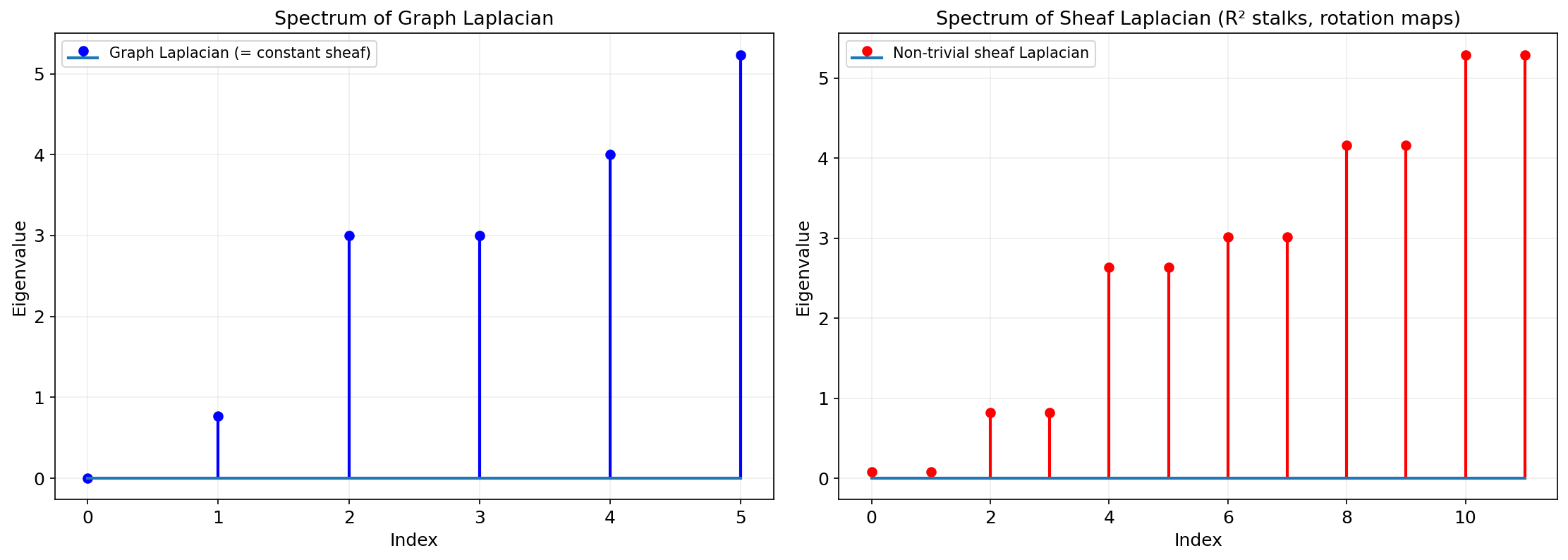
When is the constant sheaf (all stalks , all restriction maps = 1), the sheaf Laplacian reduces to the ordinary graph Laplacian . The sheaf Laplacian is a strict generalization: it allows higher-dimensional data at each node and nontrivial linear transformations along each edge.
Spectral Properties
The eigenvalues of reveal more than the graph Laplacian alone. Because the restriction maps introduce structure beyond simple connectivity, the sheaf Laplacian spectrum is generally richer — more eigenvalues, more information. (The Spectral Theorem on the Linear Algebra track guarantees that , being symmetric positive semidefinite, admits a full orthogonal eigendecomposition with real non-negative eigenvalues — the foundation on which all of the spectral analysis in this section rests.)
The smallest eigenvalue (the spectral gap) of restricted to the complement of controls the rate of convergence of sheaf diffusion and the robustness of global consistency to perturbation.
Sheaf Diffusion
Definition 9 (Sheaf Diffusion).
The sheaf diffusion process on is the ODE starting from an initial vertex assignment .
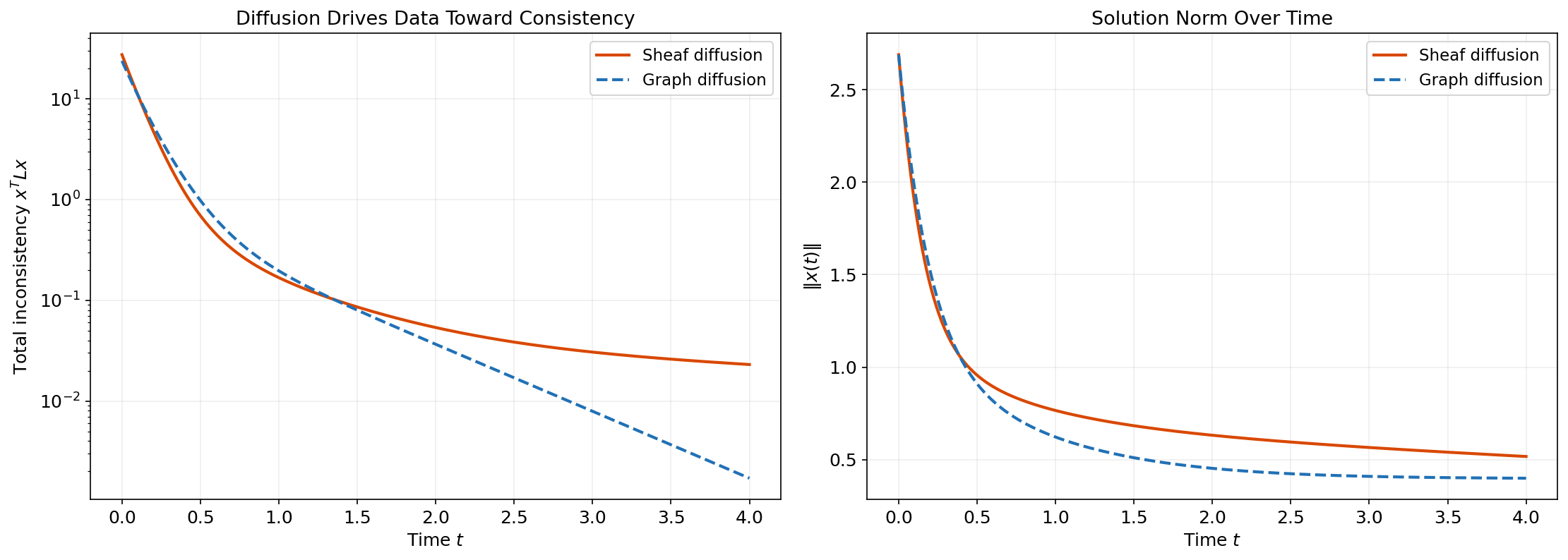
Theorem 3 (Convergence of Sheaf Diffusion).
The sheaf diffusion converges as to the orthogonal projection of onto . If is the smallest positive eigenvalue of , the convergence rate is .
Proof.
Since is symmetric positive semidefinite, it has an orthogonal eigendecomposition with . Writing , we get . As , all terms with decay exponentially, leaving only the projection onto the eigenspace, which is . The rate is controlled by .
∎In words: sheaf diffusion drives every node’s data toward the nearest globally consistent assignment. The Laplacian energy decays monotonically to zero (or to the minimum achievable with the given sheaf structure).
The simulator below lets you watch sheaf diffusion in real time. Press Play and observe how the node vectors (shown as arrows) align as the energy drops:
Sheaf diffusion drives each node's vector toward consistency with its neighbors via the restriction maps. The energy xTLFx measures total inconsistency and decays monotonically to zero.
What to notice: With the constant sheaf, all vectors converge to their average — the same consensus behavior as the heat equation on a graph. With the rotation sheaf, the convergence target depends on the rotation angle: the system finds the best compromise given the twisted compatibility conditions.
Cosheaves and Duality
A cosheaf reverses the direction of the structure maps. Where a sheaf has restriction maps from vertices to edges (projecting data down), a cosheaf has extension maps from edges to vertices (pushing data up).
Definition 10 (Cellular Cosheaf).
A cellular cosheaf on assigns:
- To each vertex , a vector space .
- To each edge , a vector space .
- To each incidence , a linear extension map .
The chain complex of a cosheaf runs in the opposite direction: , and we get cosheaf homology and .
Theorem 4 (Sheaf–Cosheaf Duality).
For a cellular sheaf on a finite graph, there is a natural dual cosheaf whose extension maps are the transposes of ‘s restriction maps. The duality is: Sheaf cohomology and cosheaf homology are dual. In particular, .
Remark.
In the Mapper algorithm, the construction that pulls back a cover and takes the nerve is naturally a cosheaf: data flows from the cover elements (edges in the nerve) to the clusters (vertices). This is the precise sense in which Mapper is a cosheaf construction — a fact that becomes visible only through the sheaf-theoretic lens.
Applications
Sensor Network Consistency
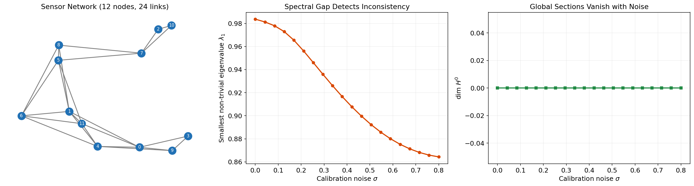
A sensor network is a graph where each vertex is a sensor and each edge represents a communication link. Each sensor measures a local quantity (temperature, position, signal strength), and the restriction maps encode the expected relationship between neighboring sensors — for instance, a rotation matrix relating two sensors’ coordinate frames.
Sheaf cohomology provides a principled consistency check:
- = number of independent consistent readings. If this equals the stalk dimension, the network is fully consistent.
- Laplacian energy = total inconsistency, interpretable as a “calibration error” across the network.
- Spectral gap = robustness of the consistency to noise. A large spectral gap means the network will recover quickly from perturbations via sheaf diffusion.
# Build a sensor network sheaf with rotation restriction maps
def build_sensor_sheaf(G, noise_level=0.0):
    """Construct a sheaf on a sensor graph with noisy rotation maps."""
    sheaf = CellularSheaf(G.nodes(), G.edges())
    for v in G.nodes():
        sheaf.set_vertex_stalk(v, 2)
    for e in G.edges():
        sheaf.set_edge_stalk(e, 2)
        theta = G.edges[e].get('angle', 0.0)
        theta_noisy = theta + noise_level * np.random.randn()
        R = np.array([[np.cos(theta_noisy), -np.sin(theta_noisy)],
                       [np.sin(theta_noisy),  np.cos(theta_noisy)]])
        sheaf.set_restriction_map(e[0], e, np.eye(2))
        sheaf.set_restriction_map(e[1], e, R)
    return sheaf
Opinion Dynamics on a Social Graph
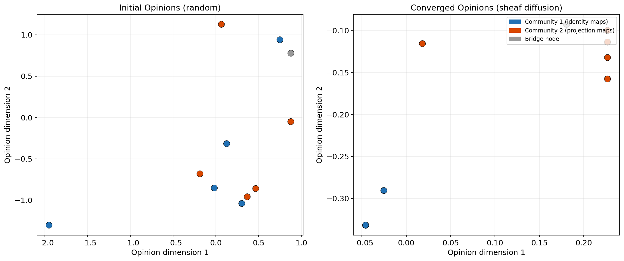
Hansen and Ghrist (2021) model opinion dynamics as sheaf diffusion. Each person (vertex) holds an opinion vector in — not just a scalar “agree/disagree” but a rich vector encoding positions on multiple issues. The restriction maps encode how people relate to each other: identity maps for people who share a frame of reference, rotation or projection maps for people who interpret the same issue differently.
Sheaf diffusion on this model drives opinions toward structured consensus — not the uniform agreement of the standard DeGroot model, but agreement modulo the restriction maps. Two people can reach “consistency” while holding different opinion vectors, as long as their opinions are related by the restriction map on the edge connecting them.
# Sheaf diffusion for opinion dynamics
def sheaf_opinion_diffusion(sheaf, x0, n_steps=100, alpha=0.1):
    """Run sheaf diffusion: x_{t+1} = x_t - α L_F x_t."""
    L = sheaf.sheaf_laplacian()
    x = x0.copy()
    trajectory = [x.copy()]
    for _ in range(n_steps):
        x = x - alpha * L @ x
        trajectory.append(x.copy())
    return np.array(trajectory)
Multi-Modal Data Fusion
When data arrives from multiple modalities — images, text, sensor readings — each modality lives in a different vector space. A cellular sheaf provides a natural framework for fusion: each modality is a vertex stalk, the relationships between modalities are restriction maps, and sheaf diffusion finds the maximally consistent joint representation.
Compared to naive fusion (e.g., concatenation or averaging), sheaf-based fusion exploits the structure of inter-modal relationships. If the restriction maps are learned from data (as in Bodnar et al., 2022), the framework becomes a sheaf neural network — a graph neural network where the message-passing rule is sheaf diffusion.
The Topology & TDA Track: A Capstone View
Remark.
With sheaf theory, we can now see how every topic in this track fits into a single algebraic framework. The table below traces the connections:
| Prior Topic | Key Concept | Sheaf-Theoretic Connection |
|---|---|---|
| Simplicial Complexes | Face poset | Cellular sheaves are functors on the face poset of a simplicial complex |
| Persistent Homology | Filtration & birth/death | Persistence modules are sheaves on the poset — the barcode is the indecomposable decomposition |
| Čech Complexes & Nerve Theorem | Nerve of a cover | Leray’s sheaf-cohomology proof of the Nerve Theorem is the original (1945) argument |
| The Mapper Algorithm | Pullback cover | Mapper’s construction is a cosheaf on the nerve: clusters push data up from edges to vertices |
| Barcodes & Bottleneck Distance | Interleaving distance | The bottleneck distance between persistence diagrams is the interleaving distance between persistence sheaves |
This is the payoff of the entire track. Each topic introduced a tool; sheaf theory reveals that they are all aspects of a single idea — local data, organized by combinatorial structure, with restriction maps governing consistency.
Where to go from here. Three frontiers extend the ideas in this track:
- Multi-parameter persistence: when the filtration parameter is two-dimensional, barcode decomposition no longer holds. The resulting persistence modules are sheaves on , and their theory is an active area of algebraic topology.
- Sheaf neural networks (Bodnar et al., 2022): replacing the graph Laplacian in a GNN with the sheaf Laplacian yields architectures that handle heterophily and avoid oversmoothing.
- Persistent sheaves: combining persistence and sheaf structure leads to sheaves parameterized by a filtration, unifying the spectral and homological perspectives.
Exercises
Foundational
Exercise 1. Let be a tree (connected graph with no cycles) and the constant sheaf with all stalks and all restriction maps . Prove that . Hint: What is the rank of the coboundary matrix for a tree with vertices?
Exercise 2. Consider a cycle graph (four vertices, four edges) with the signed sheaf: all stalks , restriction maps on three edges and on one edge. Compute and . What happens if you flip the sign on a second edge?
Exercise 3. For the complete graph with the constant sheaf ( stalks, identity maps), compute the sheaf Laplacian as an matrix. Verify that its kernel has dimension 2.
Intermediate
Exercise 4. Let be a path graph with vertex stalks and edge stalks . The restriction maps are matrices. Construct a specific example where (a one-dimensional space of global sections). What constraint does this impose on the restriction maps?
Exercise 5. Prove that the convergence rate of sheaf diffusion is exactly , where is the smallest positive eigenvalue of . Show that for the constant sheaf on a graph, equals the algebraic connectivity (second-smallest eigenvalue of the graph Laplacian).
Exercise 6. Implement the CellularSheaf class from Section 2 and verify numerically that for three different sheaves of your choice. Report the sheaf parameters and numerical results.
Advanced
Exercise 7. Sensor localization as a sheaf problem. Consider a network of 20 sensors in where each sensor knows its position relative to its neighbors (with Gaussian noise of standard deviation ). Model this as a cellular sheaf where the restriction maps are noisy rotations. Implement sheaf diffusion to estimate the global positions from local measurements. Plot the localization error as a function of and the spectral gap of .
Exercise 8. Neural sheaf diffusion. Implement a simple sheaf neural network following Bodnar et al. (2022): parameterize the restriction maps as learnable linear maps and train via gradient descent on a node classification task. Use a small graph (e.g., Karate Club) and compare accuracy with a standard GCN. Does the sheaf Laplacian improve performance on heterophilic class boundaries?
Connections
- cellular sheaves are defined on the face poset of a simplicial complex simplicial-complexes
- persistence modules are sheaves on the real line; sheaf cohomology generalizes homology to network-structured data persistent-homology
- the Nerve Theorem has a sheaf-theoretic proof via Leray's original argument cech-complexes
- Mapper's pullback-and-nerve construction is a special case of a cosheaf mapper-algorithm
- bottleneck distance generalizes to interleaving distance in the sheaf-theoretic setting barcodes-bottleneck
- the sheaf Laplacian is symmetric PSD — the Spectral Theorem guarantees its orthogonal eigendecomposition spectral-theorem
References & Further Reading
- book Topological Signal Processing — Michael Robinson (2014) The primary reference for cellular sheaves in data analysis
- paper Sheaves, Cosheaves and Applications — Justin Curry (2014) Comprehensive treatment of cellular (co)sheaves — Curry's PhD thesis
- paper Toward a Spectral Theory of Cellular Sheaves — Jakob Hansen & Robert Ghrist (2019) Spectral theory of the sheaf Laplacian
- paper Opinion Dynamics on Discourse Sheaves — Jakob Hansen & Robert Ghrist (2021) Sheaf Laplacian for opinion dynamics — the model in Section 6.2
- paper Neural Sheaf Diffusion: A Topological Perspective on Heterophily and Oversmoothing in GNNs — Bodnar, Di Giovanni, Chamberlain, Lio & Bronstein (2022) Sheaf diffusion as a graph neural network layer (ICLR 2022)
- book Elementary Applied Topology — Robert Ghrist (2014) Chapter 8 on sheaves and cosheaves — an accessible applied introduction