Information Geometry & Fisher Metric
The Fisher information metric, α-connections, and divergence functions on statistical manifolds
Overview & Motivation
The space of probability distributions is not just a set — it is a Riemannian manifold with a canonical metric. This observation, due independently to Rao (1945) and later systematized by Amari (1985), places statistical inference squarely inside the Riemannian framework we built in Riemannian Geometry and Geodesics & Curvature.
Here is the key intuition. Consider two pairs of Gaussians:
- and — the means differ by , variance is .
- and — the means differ by the same , but the variance is .
In Euclidean parameter space, these two pairs are the same distance apart: . But statistically, the second pair is far more distinguishable — a variance of means the distributions are tightly concentrated, so a shift of in the mean is enormous relative to the spread. The Fisher information metric captures this: the “true” distance between distributions depends on where you are in parameter space, exactly as a Riemannian metric varies from point to point on a manifold.
This topic brings together the three pillars of the Differential Geometry track. The parameter space of a statistical model is a smooth manifold. The Fisher information defines a Riemannian metric on this manifold. And the resulting geodesics and curvature have direct statistical meaning: geodesics are the paths of natural gradient descent, and curvature controls the precision of statistical estimation via the Cramér–Rao bound.
What We Cover
- Statistical manifolds — parametric families as smooth manifolds, identifiability, and Čencov’s uniqueness theorem
- The Fisher information metric — score functions, the Fisher matrix, and why it is a Riemannian metric
- Classical families — the Gaussian manifold as the Poincaré half-plane, Bernoulli geometry, and exponential families
- -connections — Amari’s one-parameter family, /-duality, and dually flat manifolds
- Divergence functions — KL divergence, -divergences, Bregman divergences, and the generalized Pythagorean theorem
- Geodesics — Fisher-Rao geodesics, the Mahalanobis distance, and hyperbolic geometry of variance
- The Cramér–Rao bound — curvature and estimation precision, efficient estimators
- Computational notes — symbolic Fisher metric, Christoffel symbols, geodesic solvers, natural gradient
- Information geometry in ML — natural gradient descent, variational inference, Adam, and optimal transport
Prerequisites
This topic builds directly on all three preceding topics in the Differential Geometry track:
- Smooth Manifolds — charts, tangent spaces, and the differential structure that parameter spaces inherit
- Riemannian Geometry — metric tensors, the Levi-Civita connection, parallel transport, and the machinery for measuring lengths and angles
- Geodesics & Curvature — the geodesic equation, curvature tensors, and the Gauss–Bonnet theorem
We also draw on the Spectral Theorem for eigendecomposition of the Fisher matrix, and connect to PCA & Low-Rank Approximation through the lens of preconditioning.
Statistical Manifolds & Parametric Families
Definition 1 (Statistical Model).
A parametric statistical model is a family of probability distributions on a sample space , where:
- is an open subset (the parameter space),
- The map is smooth (infinitely differentiable) for each ,
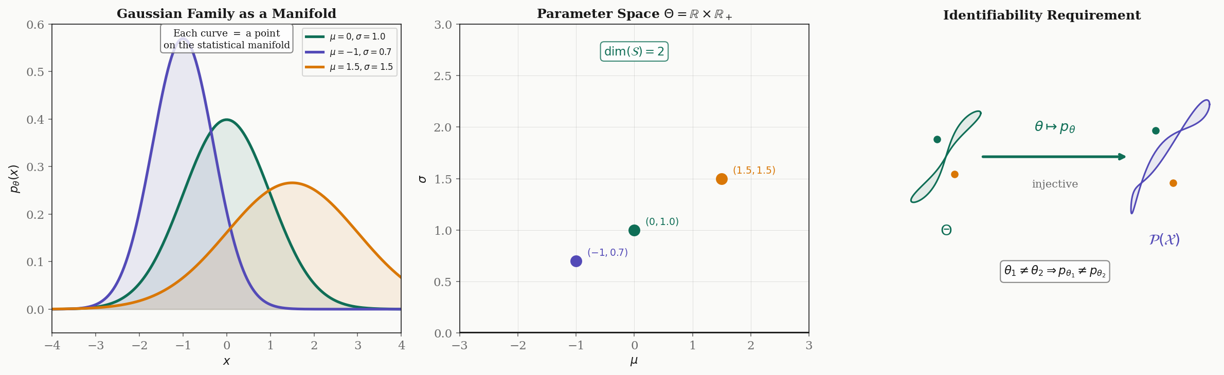
- The map is injective (identifiability): distinct parameters give distinct distributions.
Under these conditions, inherits the smooth manifold structure of . The dimension of the statistical manifold is .
The identifiability requirement (condition 3) ensures that the parameter space faithfully represents the set of distributions — there is no redundancy. Without identifiability, the Fisher metric degenerates: it becomes only positive semi-definite rather than positive definite, because some parameter directions produce no change in the distribution.
Examples. The Gaussian family has parameter space , a 2-dimensional manifold. The Bernoulli family has , a 1-dimensional manifold. The exponential family has . The multinomial on categories, with , has equal to the open -simplex.
Each point represents an entire probability distribution . As we move through the parameter space, we trace out a path through the space of distributions. The tangent space at consists of directions in which we can perturb the parameter — and, as we will see, these tangent vectors can be identified with score functions.
The Fisher Information Metric
With the smooth manifold structure in place, we now equip the parameter space with a Riemannian metric. The construction proceeds in three steps: define the score function, take its covariance, and verify that the result is a valid Riemannian metric.
Definition 2 (Score Function).
The score function of a statistical model is the gradient of the log-likelihood with respect to the parameters:
The score function measures the sensitivity of the log-likelihood to changes in the -th parameter.
Proposition 1 (Zero Mean of the Score).
For any statistical model satisfying the regularity conditions of Definition 1, the score has zero mean:
Proof.
We compute directly, using the fact that :
Interchanging the derivative and integral (justified by the smoothness assumption):
∎
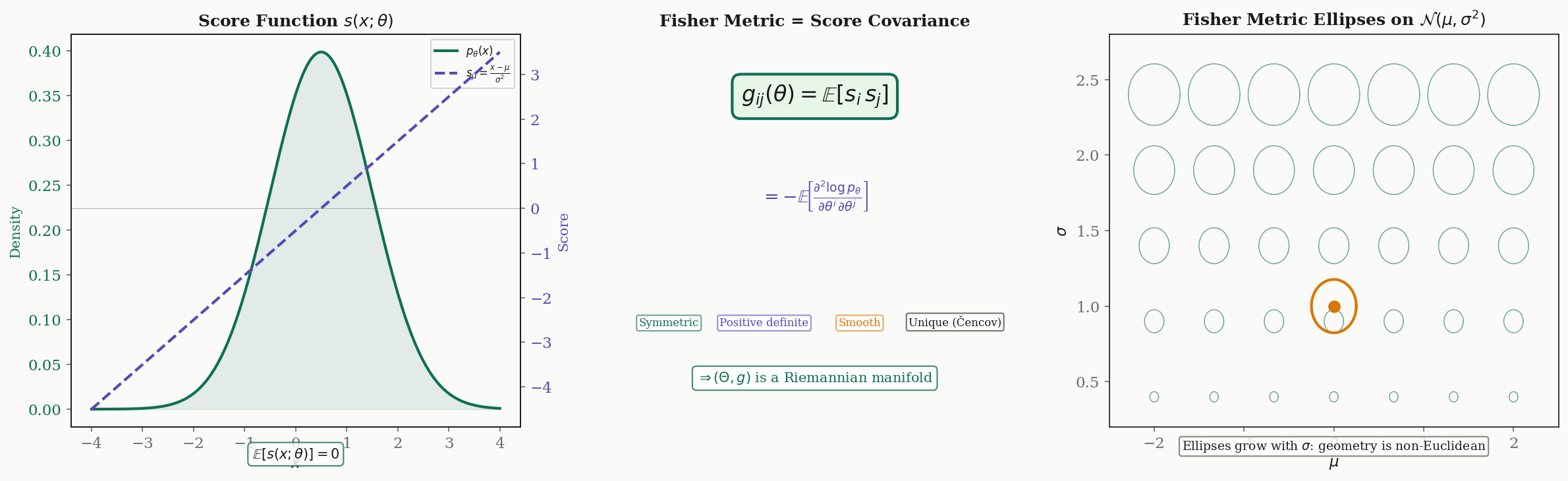
Since the score has zero mean, its covariance matrix is simply . This covariance is the Fisher information matrix.
Definition 3 (Fisher Information Matrix).
The Fisher information matrix of a statistical model is the matrix
Equivalently, under the same regularity conditions:
The equivalence of the two forms is a standard computation: differentiate the zero-mean identity with respect to and use the product rule.
Theorem 1 (Fisher Information is a Riemannian Metric).
Under the identifiability condition (Definition 1), the Fisher information matrix satisfies:
- Symmetry: (by definition, since ).
- Positive semi-definiteness: For any vector ,
- Positive definiteness: If , then for -almost all , which means a.s. By identifiability, this forces .
- Smoothness: is smooth in because is smooth.
Hence is a Riemannian manifold.
Proof.
Properties (1) and (2) are immediate from the definition. For (3), suppose . Then , so for -a.e. . This means
Exponentiating, to first order in for all directions . By identifiability, for and small , so we must have . Property (4) follows from the smoothness of and the dominated convergence theorem for the expectation integral.
∎Theorem 2 (Čencov's Uniqueness Theorem).
The Fisher information metric is the unique Riemannian metric on the space of probability distributions, up to a positive constant factor, that is invariant under sufficient statistics (Markov embeddings).
Remark (Significance of Čencov's Theorem).
We state Čencov’s theorem without proof (the full proof requires the theory of Markov kernels — see Čencov 1982). The significance is profound: the Fisher metric is not one choice among many possible Riemannian metrics on statistical manifolds. It is the canonical choice, determined uniquely by the natural invariance requirement that statistical geometry should not depend on the particular representation of the data.
Drag the point to explore how the Fisher metric varies across parameter space. Metric ellipses show the local unit ball in the Fisher metric — smaller ellipses mean higher information.
Fisher Metric for Classical Families
We now compute the Fisher metric explicitly for three canonical parametric families. Each reveals different geometric structure.
Example 1 (Gaussian Family).
For the Gaussian family with parameters :
The score functions are:
Computing the expectations :
- (by the symmetry of odd moments)
The Fisher metric is:
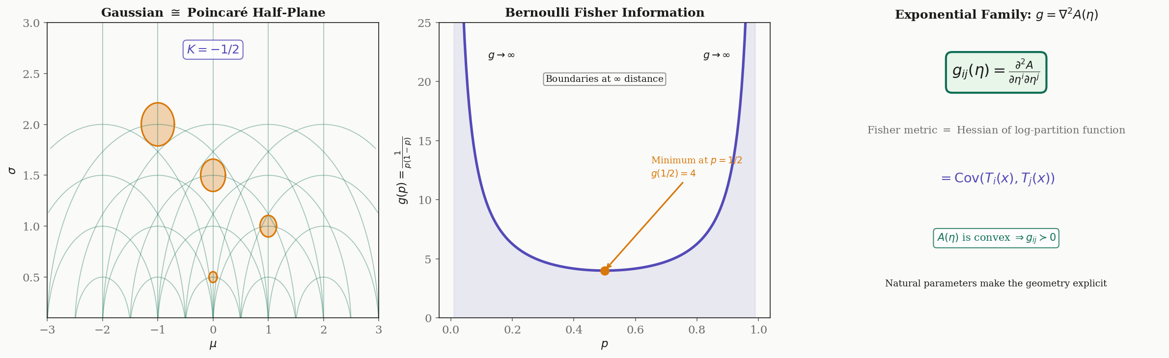
The Riemannian line element is . Up to the constant factor of in the term, this is the Poincaré upper half-plane metric on the half-plane .
Proposition 2 (Gaussian Curvature of the Gaussian Manifold).
The Gaussian family with the Fisher metric has constant negative sectional curvature .
This is computed by applying the Riemann curvature tensor formula from Geodesics & Curvature to the Fisher metric . The Gaussian manifold is a surface of constant negative curvature — a hyperbolic space. This means that the space of Gaussian distributions, equipped with the Fisher metric, has the same local geometry as the Poincaré half-plane.
Example 2 (Bernoulli Family).
For the Bernoulli family with parameter :
The score is , and the Fisher information is:
This diverges as or : the boundary of the parameter space is at infinite Fisher-Rao distance from any interior point. The Bernoulli manifold, despite being a bounded interval in Euclidean terms, is a complete Riemannian manifold of infinite diameter.
Theorem 3 (Fisher Metric for Exponential Families).
For an exponential family in natural parameters,
the Fisher metric is the Hessian of the log-partition function:
Proof.
The score function in natural parameters is:
Since (the mean parameters are the gradient of the log-partition function), the score has the form . Therefore:
For the Hessian form, differentiate again:
∎
This is a striking result: for exponential families, the Fisher metric is simply the Hessian of a single scalar function . The convexity of (a standard property of log-partition functions) guarantees positive definiteness — the Fisher metric is automatically a valid Riemannian metric.
-Connections and Dual Geometry
The Levi-Civita connection from Riemannian Geometry is the unique torsion-free, metric-compatible connection. Amari’s key insight (1985) is that statistical manifolds carry not one but a one-parameter family of connections — the -connections — and the interplay between them reveals the deepest geometric structure.
Definition 4 (α-Connection).
For , the -connection on a statistical manifold has Christoffel symbols:
where .
Special cases:
- : the Levi-Civita connection (the Riemannian geometry default)
- : the -connection (exponential connection)
- : the -connection (mixture connection)
The -connections differ from the Levi-Civita connection by a cubic tensor (the skewness tensor or Amari-Chentsov tensor) that vanishes when . The crucial property is duality.
Theorem 4 (Duality of α-Connections).
The -connection and the -connection are dual with respect to the Fisher metric:
for all vector fields on the statistical manifold.
Proof.
Write , , in local coordinates. The left side is . The right side is:
Using the definition of the -Christoffel symbols and the symmetry of the Fisher metric, the third-moment terms from and have opposite signs (the factor becomes upon negating ) and cancel in the sum. What remains is exactly the Levi-Civita compatibility equation , which holds because is metric-compatible.
∎The most important instance of duality is between the -connection () and the -connection (). This duality underlies the entire structure of exponential families.
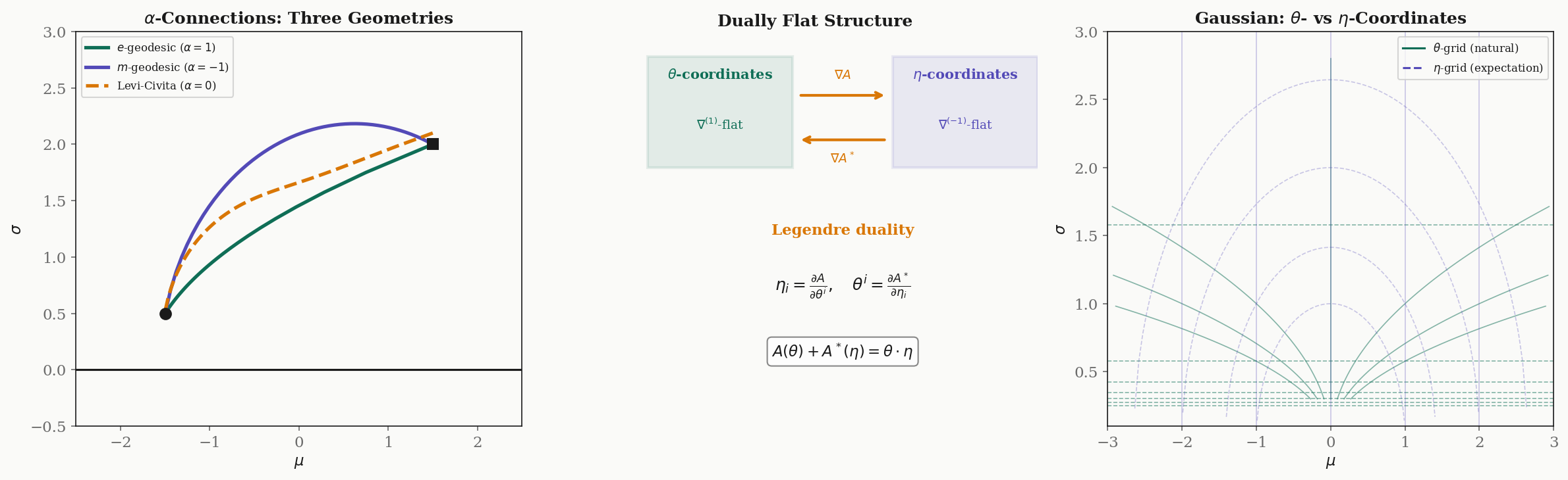
Definition 5 (Dually Flat Manifold).
A statistical manifold is dually flat if there exist coordinate systems (natural parameters) and (expectation parameters) such that:
- The -connection () is flat in -coordinates: all Christoffel symbols .
- The -connection () is flat in -coordinates: all Christoffel symbols .
- The Legendre transform links the two coordinate systems:
where is the log-partition function and is its convex conjugate.
Theorem 5 (Exponential Families are Dually Flat).
Every exponential family is a dually flat manifold. The natural parameters are -affine coordinates and the expectation parameters are -affine coordinates.
For the Gaussian family , the natural parameters are and , and the expectation parameters are and . Straight lines in -space are -geodesics; straight lines in -space are -geodesics. These are generically different curves.
Drag the two endpoints to compare geodesics under different connections. The e-geodesic is straight in natural parameters; the m-geodesic is straight in expectation parameters; the Levi-Civita geodesic (α = 0) follows the Fisher-Rao metric.
Divergence Functions
Divergence functions measure the “distance” between probability distributions, but they are not true distances — they violate symmetry and/or the triangle inequality. Nevertheless, they encode the geometry of statistical manifolds and are fundamental to inference and learning.
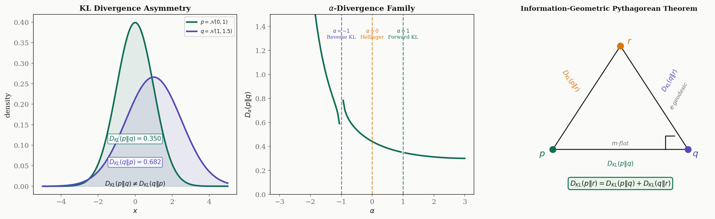
Definition 6 (KL Divergence).
The Kullback–Leibler divergence from to is:
Properties:
- (Gibbs’ inequality), with equality iff .
- in general — KL divergence is not symmetric.
- KL divergence does not satisfy the triangle inequality.
Despite not being a distance, KL divergence has a deep connection to the Fisher metric.
Proposition 3 (Fisher Metric as Hessian of KL Divergence).
The Fisher information matrix is the Hessian of the KL divergence:
Proof.
Taylor-expand around . At , the divergence is zero. The first-order term vanishes:
For the second-order term:
Thus for small . The Fisher metric is the infinitesimal KL divergence.
∎Definition 7 (α-Divergence).
The -divergence is a one-parameter family interpolating between forward and reverse KL:
Special cases:
- : (forward KL)
- : (reverse KL)
- : , twice the squared Hellinger distance
Definition 8 (Bregman Divergence).
For a strictly convex, differentiable function , the Bregman divergence is:
For exponential families, the KL divergence is a Bregman divergence with (the log-partition function):
The generalized Pythagorean theorem connects divergences to the dual geometry of -connections.
Theorem 6 (Generalized Pythagorean Theorem).
On a dually flat manifold, let , , be three distributions such that is the -projection of onto an -flat submanifold containing (i.e., the -geodesic from to is orthogonal to the -flat submanifold at ). Then:
Proof.
In a dually flat manifold, the KL divergence is a Bregman divergence: where . Expanding the right side:
The orthogonality condition says , i.e., . Using (the Legendre identity), we can simplify the sum to:
∎
This theorem is the information-geometric foundation of variational inference: minimizing over a variational family is an -projection, and the Pythagorean theorem guarantees that the optimal decomposes the divergence into an “explained” part and an irreducible “approximation error.”
Drag the two points to compare divergences between Gaussians. KL divergence is asymmetric — swapping p and q changes the value. The Fisher-Rao distance is a true metric (symmetric, triangle inequality).
Geodesics on Statistical Manifolds
The Fisher information metric defines geodesics on statistical manifolds via the geodesic equation from Geodesics & Curvature. These geodesics have concrete statistical interpretations and differ dramatically from Euclidean straight lines.
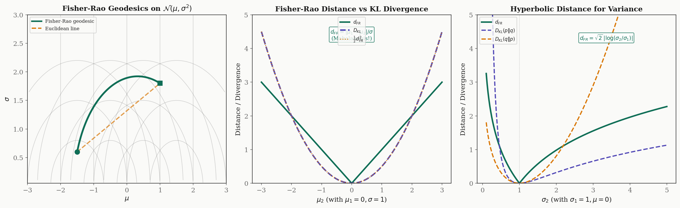
For the Gaussian family, the Fisher metric is (up to a constant) the Poincaré upper half-plane metric. The geodesics are:
- Vertical lines: , varies — changing the variance while keeping the mean fixed.
- Semicircles centered on the -axis — the shortest paths between distributions with different means and variances.
These are precisely the geodesics of hyperbolic geometry, consistent with the constant curvature .
Proposition 4 (Fisher-Rao Distance for Gaussians with Equal Variance).
For and (same variance):
This is the Mahalanobis distance.
The Fisher-Rao distance naturally produces the Mahalanobis distance — the standard “number of standard deviations” between means. This is not a coincidence: the Fisher metric is the infinitesimal Mahalanobis metric.
Proposition 5 (Fisher-Rao Distance for Gaussians with Equal Means).
For and (same mean):
Distances along the variance axis are logarithmic — the geometry is hyperbolic.
The logarithmic scaling means that doubling from to is the same Fisher-Rao distance as doubling from to . This is the natural scale for variance: what matters is the ratio, not the absolute difference.
Remark (Infinitesimal Relationship: KL and Fisher-Rao).
For infinitesimally close distributions and :
The KL divergence is the squared Fisher-Rao distance at infinitesimal scale. But for distributions that are not close, these quantities diverge: the Fisher-Rao distance is a true metric (symmetric, satisfies triangle inequality), while the KL divergence is neither.
Drag the start point to explore Fisher-Rao geodesics on the Gaussian manifold. These are semicircles in the Poincaré half-plane model.
The Cramér–Rao Bound
The Cramér–Rao bound connects the Fisher information metric to the fundamental limits of statistical estimation. It is the information-geometric version of the uncertainty principle: curvature (Fisher information) controls precision (estimator variance).
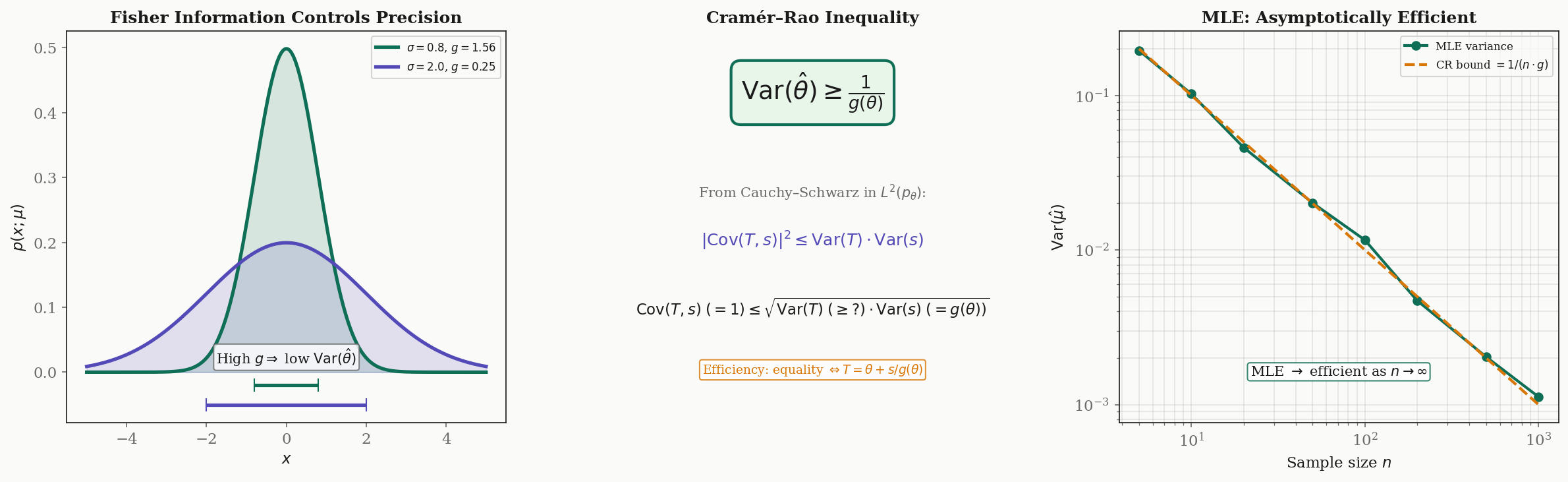
Theorem 7 (Cramér–Rao Lower Bound).
Let be an unbiased estimator of (i.e., ). Then:
More generally, for the covariance matrix of any unbiased estimator of :
where denotes the Loewner (positive semidefinite) ordering.
Proof.
We prove the scalar case using Cauchy-Schwarz in , which is precisely the inner product defined by the Fisher metric.
Since is unbiased, , so:
We compute by differentiating the unbiasedness condition:
Since , we have .
Now apply Cauchy-Schwarz:
Therefore .
∎Definition 9 (Efficient Estimator).
An unbiased estimator is efficient if it achieves the Cramér–Rao bound with equality:
Efficient estimators exist only when the score function is a linear function of . The maximum likelihood estimator (MLE) is asymptotically efficient: as the sample size , the MLE achieves the bound.
Remark (Geometric Interpretation).
The Cramér–Rao bound has a clean geometric interpretation. The Fisher metric measures the “curvature” of the log-likelihood surface:
- Large means the log-likelihood is sharply peaked — samples carry a lot of information about , so estimation is precise (low variance).
- Small means the log-likelihood is flat — samples are uninformative about , so estimation is imprecise (high variance).
The bound says: no estimator, no matter how clever, can beat the information content of the data. This is the statistical analogue of the Heisenberg uncertainty principle — but with the Fisher information playing the role of Planck’s constant.
Computational Notes
The computations of information geometry can be automated symbolically and solved numerically.
Symbolic Fisher Metric Derivation
Using SymPy, we can derive the Fisher metric for the Gaussian family from scratch:
import sympy as sp

x, mu, sigma = sp.symbols('x mu sigma', real=True)
sigma = sp.Symbol('sigma', positive=True)

# Log-likelihood
log_p = -sp.log(sigma) - (x - mu)**2 / (2 * sigma**2) - sp.log(sp.sqrt(2 * sp.pi))

# Score functions
s_mu = sp.diff(log_p, mu)          # (x - mu) / sigma^2
s_sigma = sp.diff(log_p, sigma)    # -1/sigma + (x-mu)^2 / sigma^3

# Fisher matrix entries via E[s_i * s_j]
# Using E[(x-mu)^2] = sigma^2, E[(x-mu)^4] = 3*sigma^4
g_11 = sp.Rational(1, 1) / sigma**2
g_22 = sp.Rational(2, 1) / sigma**2
g_12 = sp.Integer(0)
print(f"Fisher metric: diag({g_11}, {g_22})")
# Output: Fisher metric: diag(sigma**(-2), 2/sigma**2)
Christoffel Symbols for the Gaussian Manifold
With coordinates and metric :
# Christoffel symbols: Gamma^k_{ij} = (1/2) g^{kl}(d_i g_{jl} + d_j g_{il} - d_l g_{ij})
# For diagonal metric g = diag(f, h) where f = 1/sigma^2, h = 2/sigma^2:
# Nonzero symbols:
#   Gamma^sigma_{mu,mu}    = -f'/(2h)   = (2/sigma^3) / (2 * 2/sigma^2) = 1/(2*sigma)
#   Gamma^mu_{mu,sigma}    = f'/(2f)    = (-2/sigma^3) / (2/sigma^2) = -1/sigma
#   Gamma^sigma_{sigma,sigma} = h'/(2h) = (-4/sigma^3) / (2 * 2/sigma^2) = -1/sigma
Numerical Geodesic Solver
The geodesic equation on the Gaussian manifold is the ODE system:
We solve this with a 4th-order Runge-Kutta integrator:
import numpy as np
def geodesic_step_gaussian(state, dt):
"""Single RK4 step for the geodesic ODE on the Gaussian manifold."""
mu, sigma, dmu, dsigma = state
def derivs(s):
mu, sig, dm, ds = s
ddmu = (2 / sig) * dm * ds # -2 * Gamma^mu_{mu,sigma} * dmu * dsigma
ddsig = -dm**2 / (2*sig) + ds**2 / sig # Gamma terms
return np.array([dm, ds, ddmu, ddsig])
k1 = derivs(state)
k2 = derivs(state + 0.5*dt*k1)
k3 = derivs(state + 0.5*dt*k2)
k4 = derivs(state + dt*k3)
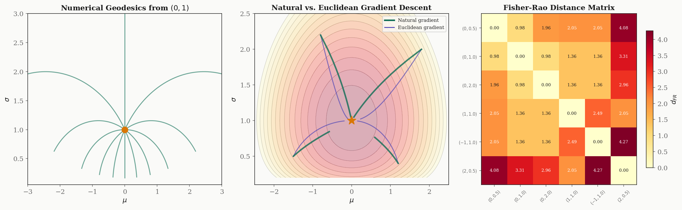
return state + (dt/6) * (k1 + 2*k2 + 2*k3 + k4)Natural Gradient Implementation
Side-by-side comparison of Euclidean and natural gradient descent minimizing :
def gradient_descent(mu, sigma, target_mu, target_sigma, lr, natural=False, steps=100):
    """Euclidean or natural gradient descent on KL divergence."""
    trajectory = [(mu, sigma)]
    for _ in range(steps):
        # Euclidean gradient of D_KL(target || model)
        grad_mu = (mu - target_mu) / sigma**2
        grad_sigma = 1/sigma - (target_sigma**2 + (target_mu - mu)**2) / sigma**3

        if natural:
            # Fisher metric inverse: g^{-1} = diag(sigma^2, sigma^2/2)
            nat_mu = sigma**2 * grad_mu
            nat_sigma = (sigma**2 / 2) * grad_sigma
            mu -= lr * nat_mu
            sigma -= lr * nat_sigma
        else:
            mu -= lr * grad_mu
            sigma -= lr * grad_sigma

        sigma = max(sigma, 0.01)  # Keep sigma positive
        trajectory.append((mu, sigma))
    return trajectory
Fisher-Rao Distance Matrix
Pairwise Fisher-Rao distances between Gaussians using Rao’s formula:
def fisher_rao_distance(mu1, s1, mu2, s2):
    """Closed-form Fisher-Rao distance for univariate Gaussians."""
    return np.sqrt(2) * np.arccosh(
        1 + ((mu1 - mu2)**2 + 2*(s1 - s2)**2) / (4 * s1 * s2)
    )
Note that this formula uses the half-plane metric , which includes the factor of in the term. The reflects the hyperbolic nature of the geometry.
Information Geometry in Machine Learning
Information geometry provides the natural mathematical framework for understanding and improving several core machine learning algorithms.
Natural Gradient Descent
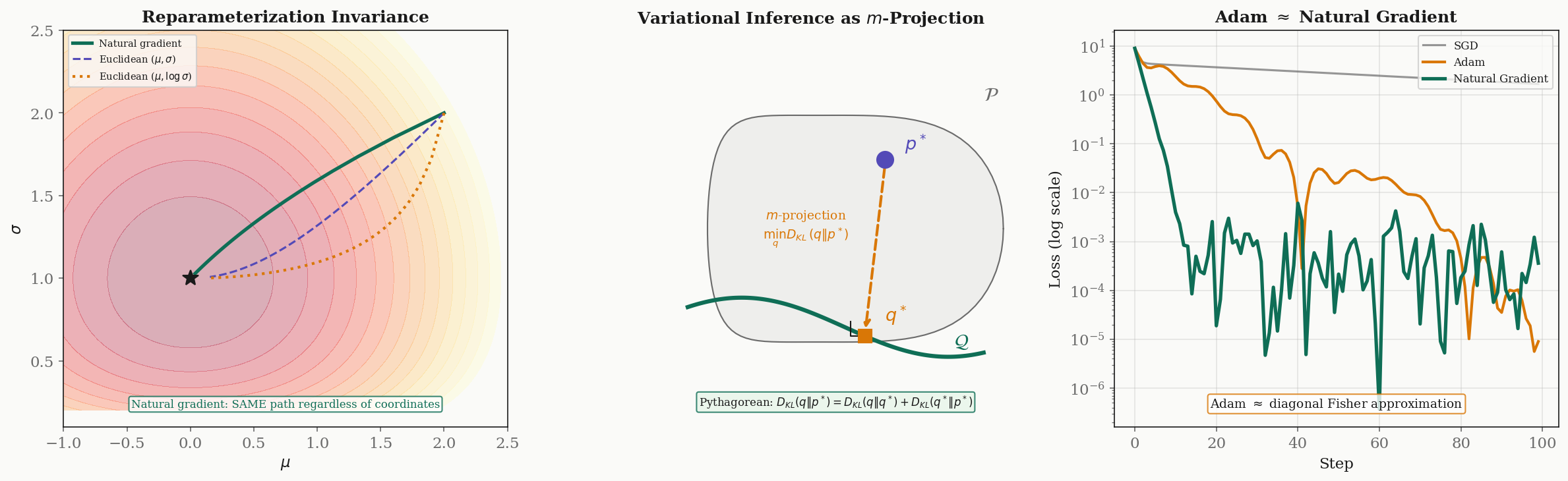
Standard gradient descent updates parameters as , using the Euclidean gradient. But the Euclidean gradient depends on the parameterization: reparameterizing the same model changes the gradient direction. This is undesirable — the “steepest descent” direction should be an intrinsic property of the model, not an artifact of how we chose to write down its parameters.
Amari’s natural gradient (1998) fixes this by using the Fisher-Rao metric:
The natural gradient is the steepest descent direction in the Riemannian metric defined by the Fisher information. It is:
- Reparameterization invariant: changing coordinates does not change the natural gradient direction (it transforms covariantly).
- Asymptotically efficient: for maximum likelihood estimation, natural gradient descent converges to the optimal rate.
- Follows geodesics approximately: the natural gradient flow traces out curves that are close to Fisher-Rao geodesics.
Variational Inference as -Projection
Variational inference minimizes over a variational family to approximate an intractable posterior . In information-geometric terms, this is the -projection of onto : the distribution in closest to in the -connection sense.
When is an exponential family (a dually flat manifold), the generalized Pythagorean theorem guarantees:
where is the optimal variational approximation. The second term is the irreducible approximation error (determined by the expressiveness of ), and the first term is what the optimization eliminates.
Adam as Approximate Natural Gradient
The Adam optimizer (Kingma & Ba, 2015) maintains running estimates of the first and second moments of the gradient. The second moment estimate is a diagonal approximation to the Fisher information matrix: . The Adam update
is therefore an approximate natural gradient step with a diagonal Fisher matrix.
K-FAC (Martens & Grosse, 2015) improves on this by using a block-diagonal, Kronecker-factored approximation to the full Fisher matrix. For a neural network layer with input and output gradient , K-FAC approximates the Fisher block as , which is far cheaper to invert than the full Fisher matrix while capturing more curvature structure than Adam’s diagonal.
Optimal Transport Connections
The Fisher-Rao metric and the Wasserstein distance define different geometries on the space of distributions:
- Fisher-Rao measures informational distance: how distinguishable are two distributions from finite samples?
- Wasserstein measures physical distance: what is the cost of transporting mass from one distribution to the other?
Otto (2001) showed that the Wasserstein space carries a formal Riemannian structure where the gradient flow of the KL divergence is the Fokker-Planck equation. The interplay between these two geometries — informational and physical — is an active research frontier connecting information geometry to optimal transport theory.
Loss Landscape Curvature
The curvature of the loss landscape at a minimum affects generalization. The “flat minima” conjecture (Hochreiter & Schmidhuber, 1997; Keskar et al., 2017) suggests that minima occupying large, flat regions of the loss surface generalize better than sharp minima. The Fisher information matrix at convergence is related to the Hessian of the loss, and its eigenspectrum characterizes the sharpness of the minimum.
Specifically, for a model trained with maximum likelihood, the Fisher information matrix equals the expected Hessian of the negative log-likelihood. The eigenvalues of at the converged parameters measure the curvature in each direction: large eigenvalues correspond to sharp directions, and the Spectral Theorem guarantees that these principal curvature directions exist and are orthogonal.
Connections & Further Reading
Information Geometry & Fisher Metric is the capstone of the Differential Geometry track. It connects back to every topic in the track and forward to applications across the curriculum:
| Connected Topic | Domain | Relationship |
|---|---|---|
| Smooth Manifolds | Differential Geometry | Parameter spaces as smooth manifolds; tangent spaces spanned by score functions |
| Riemannian Geometry | Differential Geometry | Fisher metric as Riemannian metric; Levi-Civita as connection |
| Geodesics & Curvature | Differential Geometry | Fisher-Rao geodesics; curvature for Gaussians; Gauss-Bonnet theorem |
| The Spectral Theorem | Linear Algebra | Eigendecomposition of Fisher matrix reveals principal information directions |
| PCA & Low-Rank Approximation | Linear Algebra | Natural gradient as Fisher preconditioning; covariance structure |
| Persistent Homology | Topology & TDA | Euler characteristic in Gauss-Bonnet for statistical manifolds |
| Shannon Entropy & Mutual Information | Information Theory | The entropy and mutual information quantities are developed rigorously on the Information Theory track. KL divergence is the divergence whose Hessian gives the Fisher metric. The KL divergence and its f-divergence generalizations are developed in KL Divergence & f-Divergences. |
Completing the Differential Geometry Track
With this topic, the four-part Differential Geometry track is complete:
- Smooth Manifolds (intermediate) — the foundational structure: charts, tangent spaces, and smooth maps
- Riemannian Geometry (advanced) — metric tensors, connections, and parallel transport
- Geodesics & Curvature (intermediate) — geodesic equations, curvature tensors, and the Gauss-Bonnet theorem
- Information Geometry & Fisher Metric (advanced) — the Fisher metric on statistical manifolds, -connections, and natural gradient descent
The track moves from abstract manifold structure through Riemannian geometry to the concrete, application-rich setting of statistical manifolds — where the geometric machinery built in the first three topics has direct consequences for machine learning.
Connections
- Information geometry instantiates Riemannian geometry on statistical manifolds: the Fisher metric is a specific Riemannian metric, the Levi-Civita connection is the α = 0 member of Amari's α-connection family, and parallel transport on the Gaussian manifold is parallel transport on the Poincaré half-plane. riemannian-geometry
- Statistical manifolds inherit their smooth structure from the parameter space. Charts on the Gaussian manifold are parameterizations (μ, σ) or (η₁, η₂), and the tangent space at a distribution is spanned by score functions — the derivatives of the log-likelihood. smooth-manifolds
- Fisher-Rao geodesics on the Gaussian manifold are semicircles in the Poincaré half-plane, exactly the geodesics computed by the geodesic equation. The Gaussian curvature K = -1/2 appears via the Riemann tensor machinery, and the Gauss-Bonnet theorem constrains the topology of statistical manifolds. geodesics-curvature
- The Fisher information matrix is symmetric positive definite, and its eigendecomposition reveals the principal directions of statistical information — the directions in parameter space along which estimation is most and least precise. spectral-theorem
- Natural gradient descent on the Fisher manifold is the information-geometric version of preconditioning with the Hessian. The Fisher metric plays the same role for statistical models that the covariance matrix plays for PCA: it defines the natural inner product on the parameter space. pca-low-rank
- The Euler characteristic appears in the Gauss–Bonnet theorem for statistical manifolds, connecting the topology of the parameter space to the integral of Fisher-Rao curvature — a link between topological data analysis and information geometry. persistent-homology
References & Further Reading
- book Methods of Information Geometry — Amari & Nagaoka (2000) The foundational monograph on information geometry: α-connections, duality, divergences, and applications to statistics and machine learning
- book Information Geometry and Its Applications — Amari (2016) Amari's comprehensive update covering modern applications including neural networks, machine learning, and signal processing
- book Differential-Geometrical Methods in Statistics — Amari (1985) The original Lecture Notes in Statistics volume that introduced α-connections and dually flat geometry to statistics
- paper Natural Gradient Works Efficiently in Learning — Amari (1998) Introduced natural gradient descent — steepest descent in the Fisher-Rao metric — and proved its reparameterization invariance and efficiency
- paper Information and the Accuracy Attainable in the Estimation of Statistical Parameters — Rao (1945) Rao's seminal paper introducing the Fisher information metric as a Riemannian metric on statistical manifolds — the birth of information geometry
- paper Optimizing Neural Networks with Kronecker-factored Approximate Curvature — Martens & Grosse (2015) K-FAC: practical natural gradient for deep learning using block-diagonal Kronecker-factored Fisher approximation
- paper Statistical Decision Rules and Optimal Inference — Čencov (1982) Čencov's uniqueness theorem: the Fisher metric is the unique (up to scale) Riemannian metric invariant under sufficient statistics