Riemannian Geometry
Metric tensors, connections, and parallel transport on smooth manifolds
Overview & Motivation
In the Smooth Manifolds topic, we built the language for doing calculus on curved spaces: charts, tangent vectors, the differential. But that machinery alone cannot answer the most basic geometric questions. How long is a curve on the sphere? What angle do two curves make when they cross? What is the area of a region on a surface? Smooth manifolds, by themselves, have no notion of length, angle, or volume — they are topological objects with a differentiable structure, nothing more.
The missing ingredient is a Riemannian metric: a smoothly varying inner product on each tangent space. This single piece of additional structure transforms a smooth manifold into a Riemannian manifold — a space where we can measure everything. Lengths of curves, distances between points, angles between tangent vectors, areas, volumes, curvature: all flow from the metric tensor .
Why should this matter for machine learning?
-
Natural gradient descent. The parameter space of a statistical model is a smooth manifold. The Fisher information matrix is a Riemannian metric on . Standard gradient descent ignores this geometry; natural gradient descent (Amari, 1998) uses the metric to compute steepest descent in the intrinsic sense, converging faster and more invariantly.
-
The Cramér–Rao bound. The inverse of the Fisher metric gives the minimum variance of any unbiased estimator. This is a statement about the Riemannian geometry of the parameter space.
-
KL divergence as Riemannian distance. For nearby distributions, the Kullback–Leibler divergence is the squared Riemannian distance element. Information-theoretic quantities are geometric.
What we cover. We construct the Riemannian metric and prove that every smooth manifold admits one (§2). We define curve lengths and the Riemannian distance function (§3). The musical isomorphisms — flat and sharp — bridge tangent and cotangent spaces, revealing that the gradient is metric-dependent (§4). The Fundamental Theorem of Riemannian Geometry establishes the Levi-Civita connection as the unique torsion-free, metric-compatible way to differentiate vector fields (§5). Parallel transport carries vectors along curves, and its path-dependence — holonomy — is the first shadow of curvature (§6). The Riemannian volume form enables coordinate-invariant integration (§7). Isometries and Killing vector fields capture the symmetries of a Riemannian manifold (§8). We close with computational tools (§9) and the direct connection to the Fisher information metric and natural gradient descent (§10).
Prerequisites. This topic assumes familiarity with Smooth Manifolds: charts, smooth atlases, tangent spaces , the differential , and partitions of unity. We reference the Spectral Theorem when discussing eigendecompositions of the metric tensor.
Riemannian Metrics
The central object in Riemannian geometry is a smoothly varying choice of inner product on each tangent space.
Definition 1 (Riemannian Metric).
Let be a smooth manifold. A Riemannian metric on is a smooth -tensor field such that for each point , the bilinear form is:
- Symmetric: for all .
- Positive definite: for all in .
A smooth manifold equipped with a Riemannian metric is a Riemannian manifold, denoted .
In local coordinates , the metric is represented by a matrix of smooth functions:
The inner product of two tangent vectors and is:
where we use the Einstein summation convention (repeated indices are summed). At each point, the matrix is symmetric and positive definite — which is precisely the setting of the Spectral Theorem. Its eigenvalues are the principal stretches of the metric, and its eigenvectors are the principal directions.
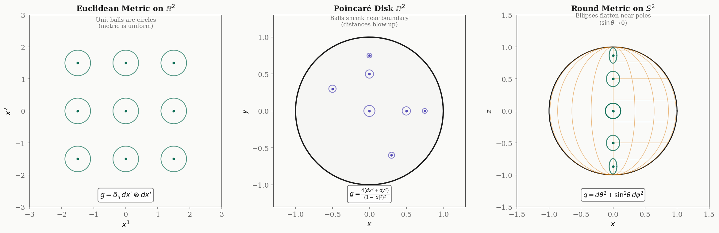
Three fundamental examples.
Example 1: The Euclidean metric on . In standard coordinates, (the identity matrix). The inner product is the ordinary dot product . The metric is the same everywhere — flat space.
Example 2: The Poincaré disk . The open unit disk with the metric:
This is a conformal metric — it is a scalar multiple of the Euclidean metric, where is the conformal factor. As a point approaches the boundary of the disk (), : distances blow up. The Poincaré disk is a model of the hyperbolic plane — a space of constant negative curvature.
Example 3: The round metric on . In spherical coordinates with (colatitude) and (azimuth):
The metric is diagonal: the -direction has unit stretching everywhere, while the -direction shrinks as near the poles. At the equator (), the metric is locally Euclidean; at the poles, the -circles collapse to points.
The natural question is: does every smooth manifold admit a Riemannian metric? The answer is yes, and the proof uses the partitions of unity from Smooth Manifolds.
Theorem 1 (Existence of Riemannian Metrics).
Every smooth manifold admits a Riemannian metric.
Proof.
Let be a smooth manifold with a smooth atlas . On each chart domain , define the pullback of the Euclidean metric:
This is a Riemannian metric on (it inherits symmetry and positive definiteness from the Euclidean inner product). Let be a smooth partition of unity subordinate to . Define:
This sum is locally finite, so is smooth. It is symmetric because each is symmetric. It is positive definite because each for , each , and at least one at each point. Therefore is a Riemannian metric on .
∎The proof is non-constructive — it tells us that metrics exist, but the particular metric we get depends on the choice of atlas and partition of unity. In practice, the metrics we work with (Euclidean, round sphere, Poincaré, Fisher) come from the geometry of the problem, not from this existence argument.
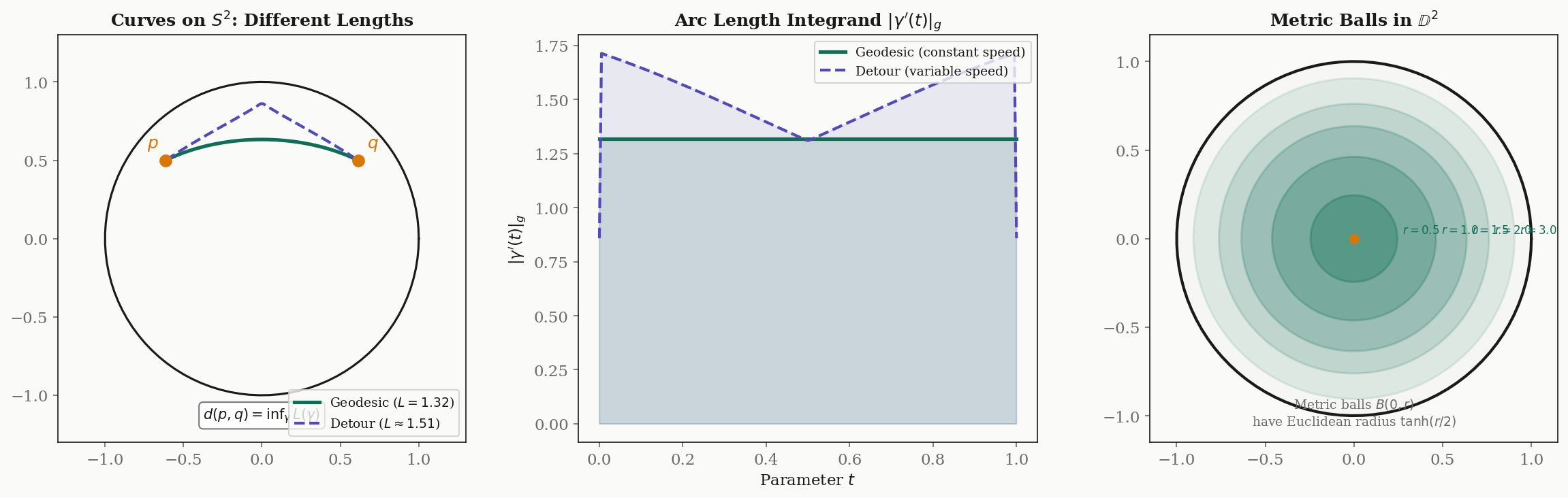
Lengths of Curves and Riemannian Distance
The metric lets us measure the length of a curve, and from curve lengths we build a distance function.
Definition 2 (Arc Length of a Curve).
Let be a piecewise smooth curve in a Riemannian manifold . The length of is:
where is the velocity vector and is the norm induced by the metric.
In local coordinates, if , this becomes:
Example. On with the round metric, a curve has length:
For the equator parametrized by with : , , , so , the circumference of a great circle.
Definition 3 (Riemannian Distance).
The Riemannian distance between two points is:
Theorem 2 (Riemannian Distance Is a Metric).
Let be a connected Riemannian manifold. The Riemannian distance is a metric on (in the metric-space sense), and the topology induced by agrees with the manifold topology.
Proof.
We verify the metric space axioms.
Non-negativity and identity of indiscernibles. is immediate since for any curve. If , the constant curve has length , so . Conversely, if , choose a chart containing but not . In this chart, is a positive-definite bilinear form, so there exist constants such that for all and in a compact neighborhood of inside . Any curve from to must exit , so its length is at least .
Symmetry. If is a curve from to , then is a curve from to with the same length. Taking the infimum over all such curves gives .
Triangle inequality. Given , concatenate a near-optimal curve from to with a near-optimal curve from to . The concatenation is a curve from to with length . Since is arbitrary, .
Topology. The comparison in each chart shows that the -balls and the Euclidean balls (pulled back to ) generate the same topology.
∎Example: great-circle distance on . For two points on the unit sphere with position vectors , the Riemannian distance is — the angle between the vectors, which is the length of the shorter great-circle arc connecting them.
Musical Isomorphisms
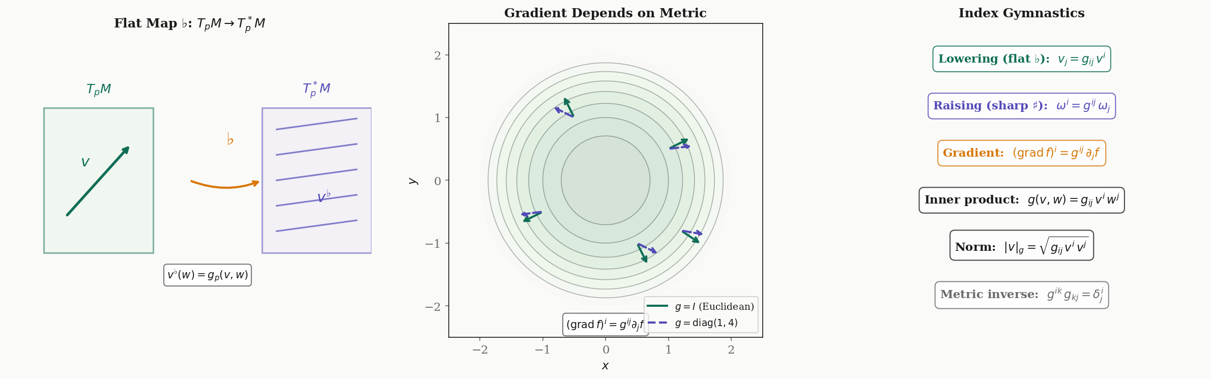
The Riemannian metric provides a canonical identification between tangent vectors and cotangent vectors — between “arrows” and “linear measurements.” This identification is called the musical isomorphisms, named for the flat () and sharp () symbols borrowed from musical notation.
Definition 4 (Flat Map (Index Lowering)).
Let be a Riemannian manifold. The flat map sends a tangent vector to the covector defined by:
In local coordinates, if , then where .
The flat map “lowers an index”: it takes a vector with an upper index and produces a covector with a lower index .
Definition 5 (Sharp Map (Index Raising)).
The sharp map is the inverse of . For a covector , the vector is defined by:
In local coordinates, if , then where and is the inverse matrix of .
Proposition 1 (Musical Isomorphisms Are Inverses).
The maps and are inverse linear isomorphisms. That is, and .
Proof.
The flat map is the linear map . Since is a non-degenerate bilinear form (positive definite implies non-degenerate), this map is injective. Since , an injective linear map between spaces of equal dimension is an isomorphism. The sharp map is defined as its inverse.
In coordinates: has components . Similarly, has components .
∎The gradient depends on the metric. Given a smooth function , the differential is a covector — it does not depend on any metric. But the gradient is a vector, and converting a covector to a vector requires the metric. In local coordinates:
In flat Euclidean space with , this recovers the familiar gradient . But on a curved manifold, the gradient depends on — change the metric, and the gradient changes direction. This is precisely why the natural gradient (which uses the Fisher information metric ) differs from the ordinary gradient (which implicitly uses the Euclidean metric).
The Levi-Civita Connection
On , differentiating a vector field is straightforward: differentiate each component. On a manifold, this does not work — the component functions live in different coordinate systems at different points, and the tangent spaces at different points are different vector spaces. To differentiate vector fields on a manifold, we need a connection: a rule for comparing tangent vectors at nearby points.
Definition 6 (Affine Connection (Covariant Derivative)).
An affine connection (or covariant derivative) on a smooth manifold is a map
satisfying, for all smooth vector fields and smooth functions :
- -linearity in :
- -linearity in :
- Leibniz rule:
The covariant derivative measures “how changes as we move in the direction ,” in a way that is well-defined on a manifold.
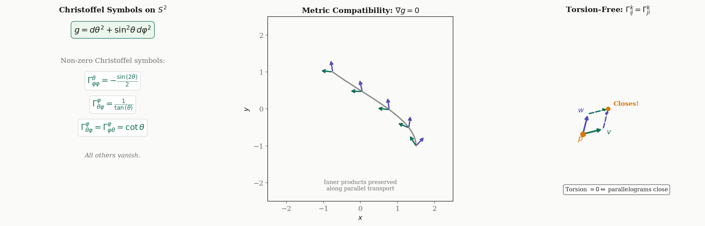
Definition 7 (Christoffel Symbols).
In local coordinates , the connection is determined by its action on coordinate basis vector fields:
The functions are the Christoffel symbols of the connection in these coordinates.
There are infinitely many possible connections on any manifold. Two additional conditions — metric compatibility and torsion-freeness — single out a unique one.
Definition 8 (Metric Compatibility).
A connection on a Riemannian manifold is metric-compatible (or compatible with the metric) if:
for all smooth vector fields . Equivalently, parallel transport preserves inner products.
Definition 9 (Torsion-Free Connection).
A connection is torsion-free (or symmetric) if:
for all smooth vector fields , where is the Lie bracket. In local coordinates, this is equivalent to the symmetry of the Christoffel symbols: .
The torsion-free condition says that infinitesimal parallelograms close: if we transport along and along , we arrive at the same point (up to the Lie bracket correction).
Theorem 3 (Fundamental Theorem of Riemannian Geometry).
On every Riemannian manifold , there exists a unique connection that is both metric-compatible and torsion-free. This connection is the Levi-Civita connection. Its Christoffel symbols are given by:
Proof.
Uniqueness. Suppose is both metric-compatible and torsion-free. We derive the Koszul formula, which determines entirely from and the Lie bracket.
Write out metric compatibility three times, cyclically permuting the arguments:
Add the first two equations and subtract the third:
Now use the torsion-free condition to replace and (and similarly for the other pairs). After collecting terms and using the symmetry of , we obtain the Koszul formula:
The right-hand side depends only on and the Lie bracket — not on . Since is non-degenerate, this formula determines uniquely. Hence at most one metric-compatible, torsion-free connection exists.
Existence. Define by the Koszul formula and verify that the result satisfies the connection axioms (linearity, Leibniz rule), metric compatibility, and torsion-freeness. This is a direct (if lengthy) computation. The Christoffel symbol formula follows by substituting , , (for which all Lie brackets vanish) and solving for using .
∎Worked example: Christoffel symbols on . With the round metric , the metric is diagonal with , , and . Since the metric components depend only on , the Christoffel symbol formula yields exactly two independent nonzero symbols (plus one symmetry partner):
All other . The first says that moving in the -direction on the sphere generates an apparent acceleration in the -direction (toward the equator). The second says that moving in the -direction while pointing in the -direction requires a correction proportional to .
| θ | φ | |
|---|---|---|
| θ | 0 | 0 |
| φ | 0 | -0.455 |
| θ | φ | |
|---|---|---|
| θ | 0 | 0.642 |
| φ | 0.642 | 0 |
Parallel Transport
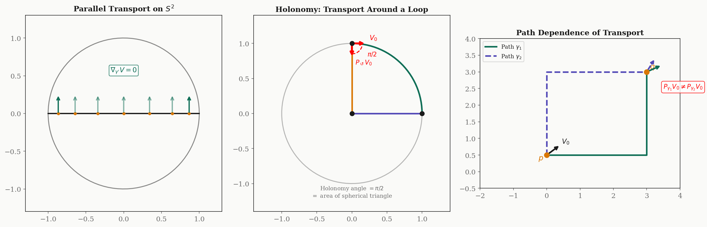
On flat , we can compare tangent vectors at different points by simply translating them. On a curved manifold, there is no canonical way to do this — the tangent spaces at different points are different vector spaces. The Levi-Civita connection provides the next best thing: we can “carry” a tangent vector along a curve while keeping it “as constant as possible.” This is parallel transport.
Definition 10 (Parallel Vector Field Along a Curve).
Let be a smooth curve in a Riemannian manifold . A vector field along is parallel if:
In local coordinates, this is the system of first-order linear ODEs:
Theorem 4 (Existence and Uniqueness of Parallel Transport).
Given a smooth curve and an initial vector , there exists a unique parallel vector field along with . The map defined by is the parallel transport along .
Proof.
In local coordinates, the parallel transport equation is a system of linear first-order ODEs with smooth coefficients (the and are smooth functions of ). By the Picard–Lindelöf theorem, the initial value problem has a unique solution on . Since the system is linear, solutions exist for all (no finite-time blowup). The solution is the unique parallel vector field, and .
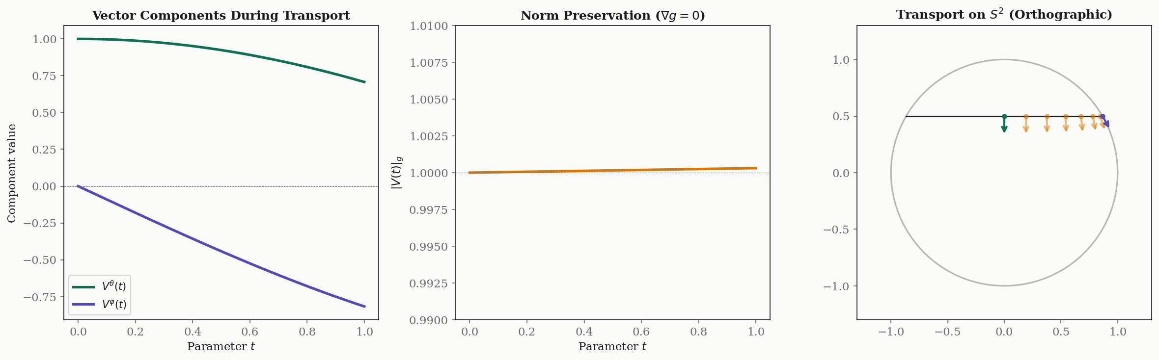
∎Proposition 2 (Parallel Transport Is a Linear Isometry).
The parallel transport map is a linear isometry:
Proof.
Let and be parallel vector fields along with and . Consider the function . Differentiating and using metric compatibility:
So is constant: .
Linearity of follows from the linearity of the ODE: if and are parallel along , then is also parallel.
∎Path dependence and holonomy. On flat , parallel transport is path-independent — the result depends only on the endpoints. On a curved manifold, parallel transport depends on the path. If we transport a vector around a closed loop back to the starting point, it generally returns rotated. The rotation angle is called the holonomy of the loop.
Example: holonomy on . Consider transporting a tangent vector around a spherical triangle with vertices at the north pole, the equator at longitude , and the equator at longitude . Each side is a geodesic (great circle arc), and the vector stays tangent to the geodesic along each side. After traversing all three sides, the vector has rotated by — exactly the solid angle subtended by the triangle ( of steradians = steradians). This is a special case of the Gauss–Bonnet theorem: on a surface of constant curvature , the holonomy of a loop enclosing area is .
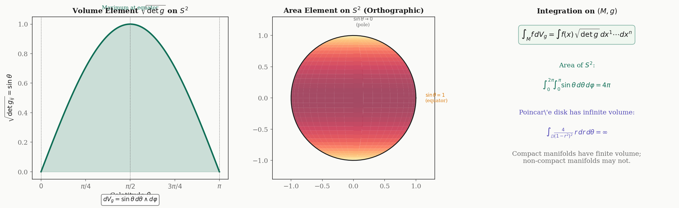
Riemannian Volume Form and Integration
The Riemannian metric determines a canonical way to measure volumes on .
Definition 11 (Riemannian Volume Form).
Let be an oriented Riemannian -manifold. The Riemannian volume form is the -form:
where is a positively oriented local coordinate system.
The factor is the Jacobian that corrects for the distortion introduced by the coordinate system. It ensures that the volume form is intrinsic — independent of the choice of coordinates.
Theorem 5 (Coordinate Independence of the Volume Form).
The Riemannian volume form is a well-defined global -form on an oriented Riemannian manifold: it does not depend on the choice of coordinates.
Proof.
Under a change of coordinates with Jacobian matrix , the metric transforms as , so . Therefore . The coordinate -form transforms as . Since the coordinates are positively oriented, , so , and the two factors cancel:
∎Worked example: area of . With the round metric , we have , so . The total area is:
For the Poincaré disk with , the volume form is . The “area” of the Poincaré disk is infinite — reflecting the fact that the hyperbolic plane has infinite extent, even though the disk looks bounded in Euclidean coordinates.
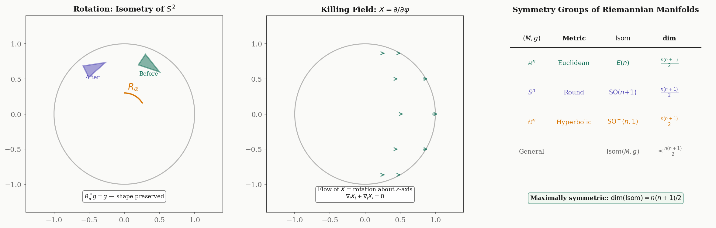
Isometries and Killing Vector Fields
Symmetries of a Riemannian manifold are the diffeomorphisms that preserve the metric.
Definition 12 (Isometry).
A diffeomorphism between Riemannian manifolds is an isometry if it preserves the metric:
Equivalently, (the pullback metric equals ). An isometry from to itself is called an isometry of .
Isometries preserve everything that depends on the metric: lengths, angles, areas, geodesics, curvature. The set of all isometries of forms a group under composition, denoted .
Examples.
- , the Euclidean group of rotations, reflections, and translations. .
- , the orthogonal group. .
- , the proper Lorentz group. Also .
Definition 13 (Killing Vector Field).
A smooth vector field on a Riemannian manifold is a Killing vector field if the flow of consists of isometries. Equivalently, satisfies Killing’s equation:
where is the Lie derivative of along , and .
Killing vector fields are the infinitesimal generators of isometries: each Killing field generates a one-parameter family of isometries. On , there are exactly three independent Killing fields — the infinitesimal rotations about the three coordinate axes — corresponding to .
Theorem 6 (Myers–Steenrod Theorem).
The isometry group of a Riemannian manifold is a Lie group. For a connected -dimensional Riemannian manifold:
A Riemannian manifold achieving equality is called maximally symmetric. The three maximally symmetric spaces of dimension are: (flat, curvature ), (positive curvature ), and (negative curvature ).
The bound decomposes as translations (or their curved analogues) plus rotations — the most symmetry any -dimensional geometry can have.
Computational Notes
The formulas in this topic are explicit enough for symbolic and numerical computation. Here we illustrate two core calculations.
Symbolic Christoffel symbols with SymPy. We can derive the Christoffel symbols for any metric directly from the formula .
import sympy as sp

theta, phi = sp.symbols('theta phi', positive=True)

# Round metric on S^2
g = sp.Matrix([[1, 0], [0, sp.sin(theta)**2]])
g_inv = g.inv()
coords = [theta, phi]

# Christoffel symbols Gamma^k_{ij}
n = 2
Gamma = [[[sp.Rational(0)] * n for _ in range(n)] for _ in range(n)]
for k in range(n):
    for i in range(n):
        for j in range(n):
            Gamma[k][i][j] = sp.Rational(1, 2) * sum(
                g_inv[k, l] * (
                    sp.diff(g[j, l], coords[i])
                    + sp.diff(g[i, l], coords[j])
                    - sp.diff(g[i, j], coords[l])
                )
                for l in range(n)
            )
            Gamma[k][i][j] = sp.simplify(Gamma[k][i][j])

# Print nonzero Christoffel symbols
for k in range(n):
    for i in range(n):
        for j in range(i, n):
            if Gamma[k][i][j] != 0:
                print(f"Gamma^{coords[k]}_{{{coords[i]},{coords[j]}}} = {Gamma[k][i][j]}")
# Output:
#   Gamma^theta_{phi,phi} = -sin(theta)*cos(theta)
#   Gamma^phi_{theta,phi} = cos(theta)/sin(theta)
Numerical parallel transport ODE. We solve numerically with forward Euler:
import numpy as np

def parallel_transport_s2(curve, curve_dot, V0, n_steps=500):
    """Parallel transport on S^2 via forward Euler."""
    dt = 1.0 / n_steps
    V = np.array(V0, dtype=float)
    trajectory = [V.copy()]

    for step in range(n_steps):
        t = step * dt
        theta, _ = curve(t)
        dgamma = np.array(curve_dot(t))
        sin_th, cos_th = np.sin(theta), np.cos(theta)

        # Christoffel symbols for S^2
        # Gamma^0_{11} = -sin(theta)*cos(theta)
        # Gamma^1_{01} = Gamma^1_{10} = cos(theta)/sin(theta)
        dV = np.zeros(2)
        dV[0] = sin_th * cos_th * dgamma[1] * V[1]  # -Gamma^0_{11} * dphi * V^phi
        dV[1] = -(cos_th / max(sin_th, 1e-10)) * (
            dgamma[0] * V[1] + dgamma[1] * V[0]
        )
        V = V + dV * dt
        trajectory.append(V.copy())

    return np.array(trajectory)

# Transport along latitude theta = pi/3, phi from 0 to pi/2
theta0 = np.pi / 3
curve = lambda t: (theta0, t * np.pi / 2)
curve_dot = lambda t: (0.0, np.pi / 2)
V0 = (1.0, 0.0)  # Initially pointing in theta-direction

result = parallel_transport_s2(curve, curve_dot, V0)

# Verify norm preservation: |V|_g should be constant
sin_th = np.sin(theta0)
norms = np.sqrt(result[:, 0]**2 + sin_th**2 * result[:, 1]**2)
print(f"Initial norm: {norms[0]:.6f}")
print(f"Final norm:   {norms[-1]:.6f}")
print(f"Max deviation: {np.max(np.abs(norms - norms[0])):.2e}")
# Output (typical):
#   Initial norm: 1.000000
#   Final norm:   0.999998
#   Max deviation: 2.14e-06
The norm is preserved to within the forward Euler truncation error — confirming metric compatibility numerically.
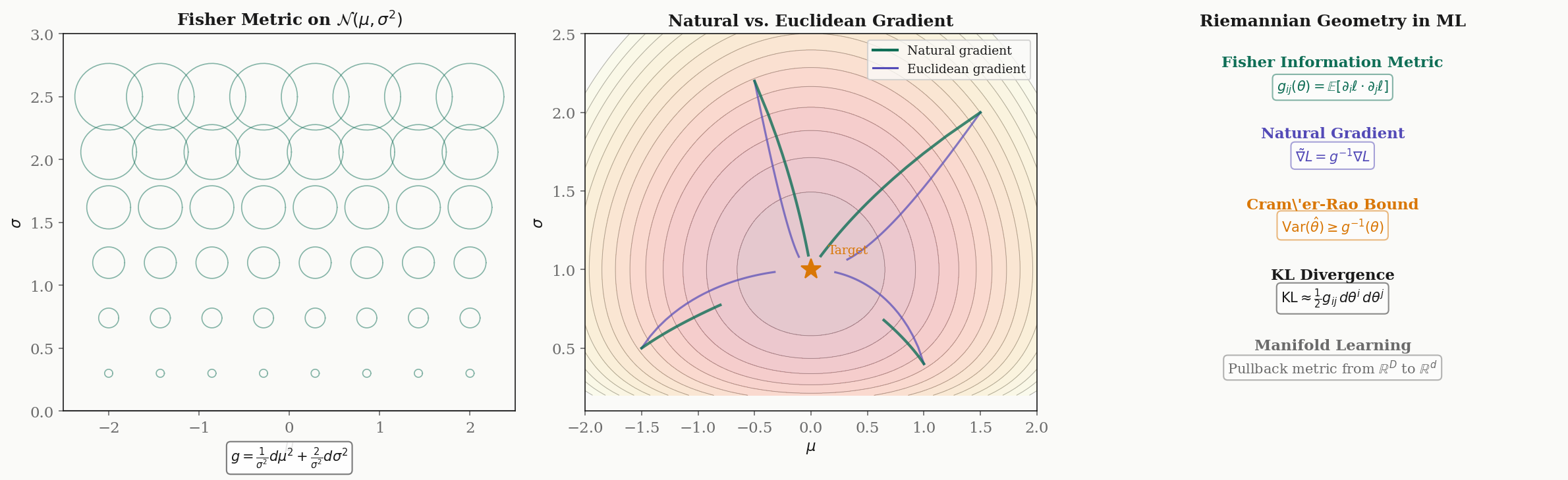
Connections to Machine Learning
The Fisher information metric turns the machinery of this topic into a tool for optimization and statistics.
The Fisher information metric. Let be a parametric family of probability distributions, with an open parameter space. The Fisher information matrix at is:
When the model is identifiable, is positive definite for all — it is a Riemannian metric on . The parameter space becomes a Riemannian manifold .
Example: Gaussian family. For with and :
The -direction is “steeper” than the -direction by a factor of — moving changes the distribution more (in the KL sense) than moving by the same Euclidean amount.
Natural gradient descent. Standard gradient descent updates using the Euclidean gradient — but this implicitly assumes the parameter space is flat with the Euclidean metric. When the parameter space is curved (which it always is for statistical models), the Euclidean gradient points in the wrong direction.
The natural gradient (Amari, 1998) uses the Fisher metric to compute the steepest descent direction in the Riemannian sense:
This is exactly the sharp map applied to the Euclidean gradient: . The natural gradient is invariant under reparametrization — it does not depend on the coordinates we use for .
KL divergence as Riemannian distance. For nearby parameters and :
The KL divergence is the squared infinitesimal Riemannian distance. This is why the Fisher metric is natural: it is the unique Riemannian metric (up to scale) for which KL divergence is the distance.
The Cramér–Rao bound. For any unbiased estimator of :
The inverse Fisher metric is the lower bound on estimation variance. The metric tells us how hard it is to distinguish nearby parameters — directions where is large are “easy” to estimate (the distributions are very different); directions where is small are “hard.”
Connections and Further Reading
Cross-topic connections.
| Topic | Connection |
|---|---|
| Smooth Manifolds | The prerequisite: charts, tangent spaces, and the differential are the raw inputs for Riemannian geometry. The metric is the additional structure that enables measurement. |
| The Spectral Theorem | The metric tensor at each point is symmetric positive definite — its eigendecomposition reveals the principal directions and magnitudes of the metric. |
| Singular Value Decomposition | The differential of a map between Riemannian manifolds decomposes via SVD into rotations and stretches. The singular values measure metric distortion. |
| PCA & Low-Rank Approximation | Local PCA on data near a manifold estimates the tangent space metric. The Riemannian metric is the theoretical foundation for manifold learning. |
Where this leads.
-
Geodesics & Curvature — The Levi-Civita connection defines geodesics as curves with zero acceleration (). The Riemann curvature tensor measures the failure of parallel transport to be path-independent. Sectional curvature, Ricci curvature, and scalar curvature each capture different aspects of how the manifold curves.
-
Information Geometry & Fisher Metric — The Fisher information metric on statistical manifolds, natural gradient methods for neural network optimization, -connections, and the geometry of exponential families. This topic provides the complete Riemannian foundation; Information Geometry builds the statistical superstructure.
Connections
- Riemannian geometry builds directly on smooth manifolds by adding an inner product to each tangent space. Charts, tangent vectors, and the differential from the Smooth Manifolds topic are the raw inputs; the Riemannian metric is the additional structure that makes geometric measurement possible. smooth-manifolds
- The metric tensor g_ij at each point is a symmetric positive-definite matrix. Its eigendecomposition — the Spectral Theorem — reveals the principal directions and magnitudes of the metric, determining how the manifold stretches and compresses in each direction. spectral-theorem
- The Jacobian of a smooth map between Riemannian manifolds decomposes via SVD into stretching (singular values) and rotational components. In Riemannian geometry, this decomposition of the differential dF_p reveals how the map distorts the metric. svd
- PCA on data sampled near a manifold estimates the tangent space metric locally. The Riemannian metric provides the theoretical foundation for local PCA methods and manifold learning algorithms that respect the intrinsic geometry of the data. pca-low-rank
References & Further Reading
- book Riemannian Manifolds: An Introduction to Curvature — Lee (2018) Chapters 2-5: The primary graduate reference for Riemannian metrics, connections, and geodesics. Second edition (Riemannian Manifolds: An Introduction to Curvature → Introduction to Riemannian Manifolds).
- book Semi-Riemannian Geometry with Applications to Relativity — O'Neill (1983) Chapters 3-5: Classical treatment of connections, parallel transport, and curvature with applications to general relativity
- book Differential Geometry: Connections, Curvature, and Characteristic Classes — Tu (2017) Chapters 2-6: Accessible treatment connecting Riemannian geometry to vector bundles and characteristic classes
- book Foundations of Differential Geometry, Vol. I — Kobayashi & Nomizu (1963) Chapters II-IV: Affine connections, parallel transport, and curvature — the classical definitive reference
- paper Natural Gradient Works Efficiently in Learning — Amari (1998) Foundational paper connecting Riemannian geometry (Fisher information metric) to neural network optimization
- paper Information Geometry and Its Applications — Amari (2016) Comprehensive treatment of the Fisher information metric as a Riemannian metric on statistical manifolds