Geodesics & Curvature
Geodesic equations, curvature tensors, and the Gauss–Bonnet theorem
Overview & Motivation
In Riemannian Geometry, we equipped smooth manifolds with a metric tensor and built the Levi-Civita connection — the unique torsion-free, metric-compatible covariant derivative. With this machinery, we could measure lengths, angles, and areas, and we could parallel-transport vectors along curves. But we left the most fundamental geometric questions unanswered: what are the “straight lines” on a curved space? How do we quantify how much a manifold deviates from being flat? And what are the global consequences of local curvature?
This topic answers all three. Geodesics are the curves of zero acceleration — the closest thing to straight lines on a Riemannian manifold. On the sphere , they are great circles; on the hyperbolic plane, they are semicircles orthogonal to the boundary in the Poincaré disk model. The geodesic equation is a system of second-order ODEs whose solutions encode the manifold’s intrinsic geometry, and the exponential map packages these solutions into a smooth map from each tangent space to the manifold.
The Riemann curvature tensor measures the failure of parallel transport to be path-independent. Its contractions — sectional, Ricci, and scalar curvature — capture progressively coarser geometric information, from the curvature of individual 2-planes to a single scalar summary at each point.
The climax is the Gauss–Bonnet theorem: the total Gaussian curvature of a closed surface equals , where is the Euler characteristic. This is a profound bridge between local geometry (curvature at each point) and global topology (the shape of the manifold as a whole). You can deform a sphere into any potato-shaped blob, and the total curvature remains — because the Euler characteristic is a topological invariant, computable via the Betti numbers from Persistent Homology or the formula from Simplicial Complexes.
Jacobi fields describe how nearby geodesics spread or converge, with the sign of curvature controlling the behavior. Positive curvature focuses geodesics (like meridians on a sphere converging at the poles); negative curvature causes exponential divergence (like geodesics on a saddle surface). The comparison theorems — Bonnet–Myers, Cartan–Hadamard, Rauch, and Bishop–Gromov — draw sweeping global conclusions from curvature bounds.
For machine learning, curvature appears in manifold learning (the curvature of data manifolds determines how well local linear approximations work), natural gradient descent (geodesics in the Fisher metric parameter space), loss landscape analysis (flat minima generalize better than sharp ones), and graph analysis (Ollivier–Ricci curvature detects community structure).
What We Cover
- Geodesics — the geodesic equation, existence and uniqueness, constant speed, great circles on
- The exponential map — normal coordinates, the injectivity radius, curvature at second order
- The Riemann curvature tensor — definition, coordinate formula, symmetries, flatness criterion
- Sectional, Ricci, and scalar curvature — the contraction hierarchy, Schur’s lemma
- The Gauss–Bonnet theorem — angle excess, the global theorem, topological constraints
- Jacobi fields — the Jacobi equation, conjugate points, curvature and geodesic deviation
- Comparison theorems — Bonnet–Myers, Cartan–Hadamard, Rauch, Bishop–Gromov
- Computational notes — symbolic Riemann tensor computation, numerical geodesic solvers
- Curvature in ML — manifold learning, natural gradient, loss landscapes, graph Ricci curvature
Prerequisites
This topic builds directly on Riemannian Geometry. We use the Levi-Civita connection and its Christoffel symbols throughout — these enter the geodesic equation, the Riemann tensor formula, and the Jacobi equation. Parallel transport from that topic is exactly what curvature measures the path-dependence of. The Smooth Manifolds foundation (charts, tangent spaces, the differential) provides the underlying language.
Geodesics: Curves of Zero Acceleration
On a Riemannian manifold with the Levi-Civita connection , a geodesic is a curve whose velocity vector is parallel along itself — it has zero covariant acceleration.
Definition 1 (Geodesic).
Let be a Riemannian manifold with Levi-Civita connection . A smooth curve is a geodesic if
Equivalently, parallel-transports its own velocity vector.
The definition says that geodesics are “unaccelerated” — not that they are the shortest paths (though they locally are). Think of a geodesic as what you get when you walk forward without turning: you follow the curvature of the manifold, but you never steer.
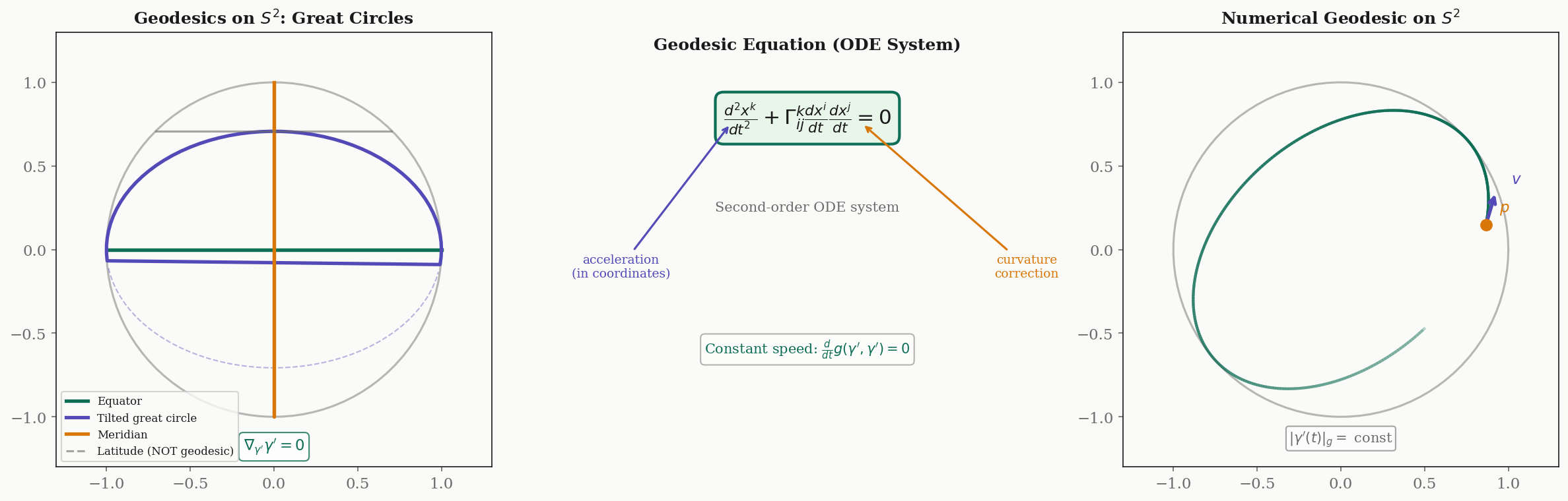
In local coordinates , writing out using the Christoffel symbols gives the geodesic equation:
where and . This is a system of second-order ODEs — the Christoffel symbols act as “correction terms” that account for the curvature of the coordinate system. On flat with Cartesian coordinates, all and the geodesic equation reduces to : straight lines.
Example: great circles on . On the unit sphere with the round metric , the nonzero Christoffel symbols are and . The geodesic equation becomes:
The solutions are exactly the great circles — intersections of the sphere with planes through the origin. The equator , is the simplest example: the first equation gives and the second gives .
The geodesic equation is a second-order ODE, and the standard existence-uniqueness theorem from ODE theory applies immediately.
Theorem 1 (Existence and Uniqueness of Geodesics).
Let be a Riemannian manifold, , and . There exists a unique maximal geodesic (where is the largest open interval containing ) such that and .
The word maximal means we extend the geodesic as far as it will go. On a compact manifold like , every geodesic extends to all of . On an incomplete manifold (like with a point removed), a geodesic may “fall off the edge” in finite time. A Riemannian manifold is complete if every geodesic extends to all of — equivalently, by the Hopf–Rinow theorem, if it is complete as a metric space.
An immediate consequence of the geodesic equation and the metric compatibility of is that geodesics travel at constant speed.
Proposition 1 (Geodesics Have Constant Speed).
If is a geodesic, then is constant.
Proof.
We compute the derivative of the squared speed:
where we used: (1) metric compatibility of , which gives ; and (2) the geodesic condition . Since is constant, so is .
∎Constant speed means we can parametrize geodesics by arc length without reparametrization. A geodesic with is a unit-speed geodesic, and the parameter measures the distance traveled along the curve.
The Exponential Map & Normal Coordinates
The exponential map packages the initial-value problem for geodesics into a single smooth map from each tangent space to the manifold.
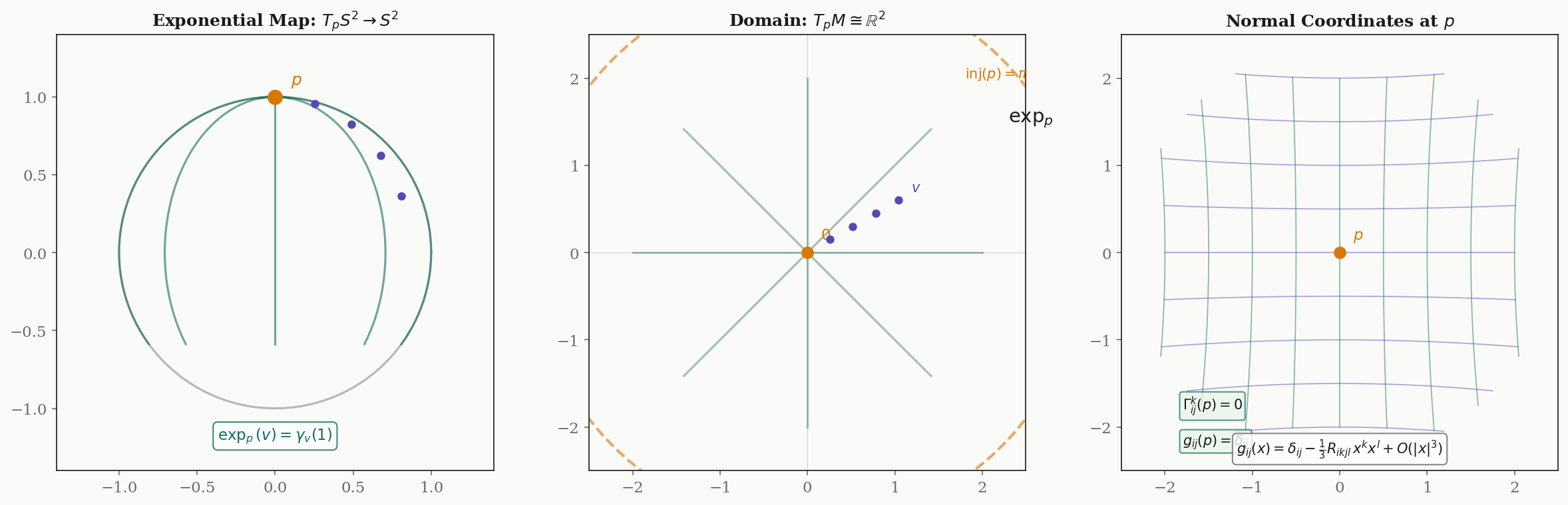
Definition 2 (Exponential Map).
Let be a Riemannian manifold and . For such that the geodesic with and is defined at , the exponential map at is
where is the set of all such .
The name “exponential” comes from Lie group theory: for matrix Lie groups, the Riemannian exponential map coincides with the matrix exponential. The key observation is the rescaling property: . So the geodesic in the direction is the image of the ray in the tangent space under . Straight lines through the origin in map to geodesics through in .
Theorem 2 (Normal Neighborhood Theorem).
For each , there exists such that maps the open ball diffeomorphically onto an open neighborhood of in .
Proof.
The differential of at the origin is the identity: . This follows because for any :
Since is invertible, the inverse function theorem guarantees that is a local diffeomorphism near .
∎This theorem is the gateway to a particularly nice coordinate system.
Definition 3 (Normal Coordinates).
Let be an orthonormal basis for . The normal coordinates (or Riemannian normal coordinates) at are the coordinates defined by
for in a normal neighborhood of .
Normal coordinates have remarkable properties at the center point :
- The metric is Euclidean: .
- Christoffel symbols vanish: .
- Geodesics through are straight lines: in these coordinates.
- Curvature appears at second order: .
The last property is the most profound: to first order, every Riemannian manifold looks Euclidean. The deviation from flatness is controlled by the Riemann curvature tensor, and it appears only at second order. This is why we needed the full machinery of connections and curvature tensors — first-order information cannot distinguish a curved manifold from a flat one.
Definition 4 (Injectivity Radius).
The injectivity radius at is
The injectivity radius of is .
On the unit sphere , the injectivity radius at every point is — the antipodal point. Geodesics from the north pole are great circles that converge at the south pole (distance ), and is a diffeomorphism on the open hemisphere of radius . Beyond , the exponential map is no longer injective: multiple geodesics from reach the same point.
The Riemann Curvature Tensor
With geodesics and the exponential map in hand, we now attack the central question: how do we measure the curvature of a Riemannian manifold? The answer is the Riemann curvature tensor — a -tensor that captures everything about the intrinsic curvature.
Definition 5 (Riemann Curvature Endomorphism).
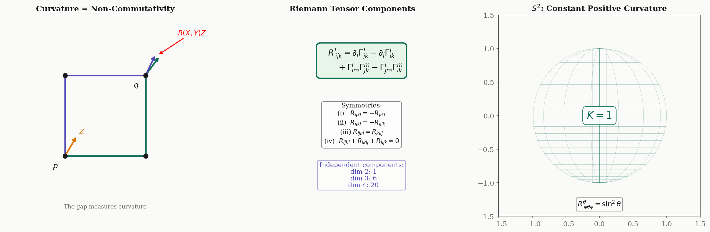
The Riemann curvature endomorphism is the -tensor field defined by
for smooth vector fields on .
The definition looks abstract, but the geometric meaning is concrete: measures the failure of parallel transport to be path-independent. If we parallel-transport first in the direction, then in the direction, versus first in then in , the results differ by exactly (after correcting for the Lie bracket term). On flat , parallel transport is path-independent, and identically.
In local coordinates, the components are computed from the Christoffel symbols:
The fully covariant Riemann tensor has a rich set of symmetries that drastically reduce the number of independent components.
Theorem 3 (Symmetries of the Riemann Tensor).
The Riemann curvature tensor satisfies:
- Skew symmetry in the first pair:
- Skew symmetry in the second pair:
- Pair symmetry:
- First Bianchi identity:
These symmetries reduce the number of independent components from to .
Proof.
We prove the first Bianchi identity. Let , , be vector fields. By definition of and the torsion-free property of the Levi-Civita connection (), we compute:
Using the torsion-free property to replace Lie brackets , all terms cancel in pairs. The key step is that each term appears once with a plus sign and once with a minus sign in the cyclic sum, and the bracket correction terms supply the missing cancellations. The detailed computation requires expanding all nine terms and checking that they cancel; we omit the bookkeeping but the mechanism is the torsion-free property applied systematically.
∎The component count formula gives concrete numbers: in dimension 2, there is exactly 1 independent component (the manifold’s curvature is determined by a single function). In dimension 3, there are 6. In dimension 4 (spacetime in general relativity), there are 20.
The Riemann tensor provides a complete local characterization of flatness.
Theorem 4 (Flatness Criterion).
A Riemannian manifold is locally isometric to Euclidean space if and only if everywhere. Equivalently, if and only if parallel transport is path-independent in some neighborhood of every point.
This theorem closes the circle: the Riemann tensor is the complete obstruction to flatness. A manifold with is locally indistinguishable from — though it may still be globally different (a flat torus has but is not diffeomorphic to ).
Sectional, Ricci, and Scalar Curvature
The full Riemann tensor carries a lot of information — in dimension , it has independent components. We extract scalar-valued curvature quantities by successively contracting indices, creating a hierarchy from most to least informative.
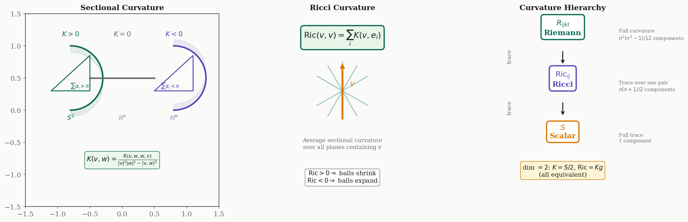
Definition 6 (Sectional Curvature).
For a 2-dimensional subspace (2-plane) , the sectional curvature is
The denominator is the squared area of the parallelogram spanned by and , ensuring depends only on the plane , not on the choice of spanning vectors.
Sectional curvature has a clean geometric interpretation: is the Gaussian curvature of the 2-dimensional surface formed by geodesics tangent to at . The spaces of constant sectional curvature are the most symmetric Riemannian manifolds:
- : (positive constant — the sphere)
- : (flat — Euclidean space)
- : (negative constant — hyperbolic space)
Definition 7 (Ricci Curvature).
The Ricci curvature is the trace of the Riemann curvature endomorphism over one pair of indices:
where is an orthonormal basis for .
The Ricci curvature averages the sectional curvatures of all 2-planes containing . It governs volume comparison: positive Ricci curvature means geodesic balls grow more slowly than in flat space (this is the content of the Bishop–Gromov theorem in §8).
Definition 8 (Scalar Curvature).
The scalar curvature is the full trace of the Ricci tensor:
It is a single real number at each point — the coarsest curvature invariant.
The contraction hierarchy from most to least informative:
Each contraction loses information. The full Riemann tensor determines both Ricci and scalar curvature, but not vice versa (except in low dimensions). In dimension 2, all three are equivalent: and , so the single Gaussian curvature function contains all curvature information.
A natural question: if the sectional curvature at each point happens to be the same for all 2-planes (but may vary from point to point), does it follow that is actually constant on all of ? In dimension , the answer is yes.
Proposition 2 (Schur's Lemma).
If and the sectional curvature at each point depends only on (not on the choice of 2-plane ), then is constant on all of .
Proof.
The assumption says for all 2-planes . This is equivalent to the Riemann tensor having the special form . Taking the covariant divergence and using the second Bianchi identity (contracted form), we obtain where . Since , the coefficient , and therefore , meaning is constant. (This argument fails in dimension 2, where ; indeed, surfaces can have non-constant Gaussian curvature.)
∎The Gauss–Bonnet Theorem
The Gauss–Bonnet theorem is the crown jewel of two-dimensional Riemannian geometry. It connects local geometry (the Gaussian curvature at each point) to global topology (the Euler characteristic of the manifold). This is a paradigmatic result in the broader theme of “index theorems” that relate analytic and topological data.
We start with the local version, which is elementary and beautiful.
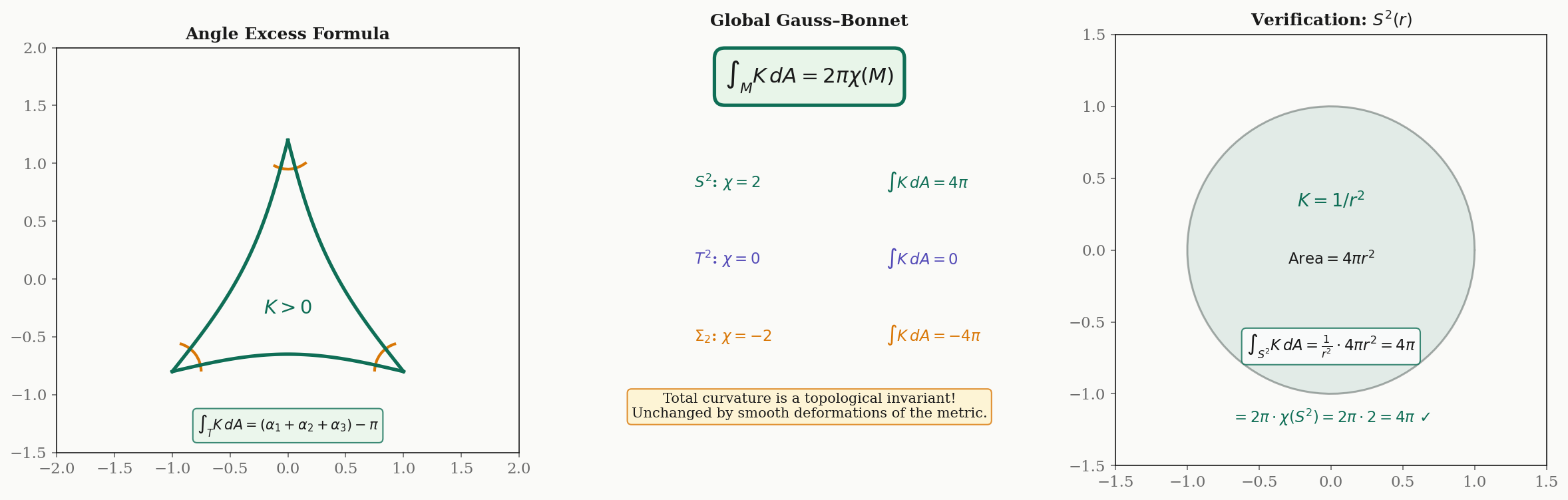
Theorem 5 (Local Gauss–Bonnet (Angle Excess)).
Let be a geodesic triangle on a Riemannian surface with interior angles . Then
Proof.
The proof uses Green’s theorem on the manifold. Consider the geodesic triangle with vertices and edges that are geodesic segments. The geodesic curvature of each edge is zero (because the edges are geodesics). By the general Gauss–Bonnet formula for a region with piecewise smooth boundary:
where is the geodesic curvature of the boundary and are the exterior angles at the vertices. Since along geodesic edges, we get .
∎This is the angle excess formula: the integral of curvature over a geodesic triangle equals the deviation of the angle sum from .
- Positive curvature (): Angles sum to more than — “fat” triangles. On a sphere, a geodesic triangle with three right angles () has angle sum , and the area of this triangle is times .
- Zero curvature (): Angles sum to exactly — Euclidean geometry.
- Negative curvature (): Angles sum to less than — “thin” triangles.
The global version integrates over the entire manifold.
Theorem 6 (Global Gauss–Bonnet).
Let be a compact oriented Riemannian 2-manifold without boundary. Then
where is the Euler characteristic of .
The Euler characteristic is a topological invariant: , , and for a surface of genus . (Recall from Simplicial Complexes that for any triangulation, and from Persistent Homology that via the alternating sum of Betti numbers.)
The consequences are immediate and powerful:
- cannot carry a flat metric. Since , any metric on must have , so cannot vanish everywhere.
- The torus admits a flat metric. Since , the total curvature of any metric on is zero. Positive curvature on the outer edge of a torus is exactly cancelled by negative curvature on the inner edge.
- Surfaces of genus cannot have everywhere. Since for , the total curvature is negative, which forces somewhere.
- Total curvature is a topological invariant. You can deform the metric however you like — stretch, compress, bend — and remains unchanged. The geometry changes; the topology does not.
Remark. The Gauss–Bonnet theorem generalizes to higher even dimensions as the Chern–Gauss–Bonnet theorem. In dimension , the integrand is the Pfaffian of the curvature form rather than the scalar curvature. The 2-dimensional case is special because the Pfaffian reduces to the Gaussian curvature .
Jacobi Fields & Geodesic Deviation
Geodesics tell us about single paths on a manifold. To understand the geometry around a geodesic — how neighboring geodesics behave — we study Jacobi fields.
Definition 9 (Jacobi Field).
Let be a geodesic on . A vector field along is a Jacobi field if it satisfies the Jacobi equation:
The geometric meaning: consider a one-parameter family of geodesics with . The variation vector is a Jacobi field along . So Jacobi fields describe the infinitesimal deviation between nearby geodesics.
The Jacobi equation is a second-order linear ODE along . Since the initial data live in the -dimensional tangent space, the space of Jacobi fields along is -dimensional.
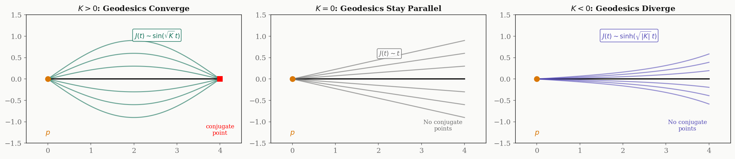
The sign of sectional curvature determines Jacobi field behavior. This is the key geometric insight. For a space of constant sectional curvature , the Jacobi equation has explicit solutions. If and (a unit vector perpendicular to ), then equals:
| Curvature | Jacobi field norm | Behavior |
|---|---|---|
| Oscillates — geodesics converge | ||
| Linear growth — geodesics spread steadily | ||
| Exponential growth — geodesics diverge |
Positive curvature focuses geodesics: neighboring geodesics starting parallel will eventually cross. Negative curvature defocuses them: neighbors diverge exponentially.
Definition 10 (Conjugate Point).
A point is conjugate to along if there exists a non-zero Jacobi field with and .
At a conjugate point, a family of geodesics from “refocuses” — the envelope of nearby geodesics passes through zero. On , the conjugate point to the north pole along any geodesic is the south pole at distance (where every meridian meets).
Conjugate points mark the boundary of where geodesics are optimal.
Theorem 7 (Geodesics Do Not Minimize Past Conjugate Points).
Let be a geodesic from with a conjugate point . Then does not minimize length past : for any , there exists a shorter curve from to .
Proof.
The idea is to construct a variation that shortens the geodesic. Let be the Jacobi field with and . Because and is non-zero, the family of geodesics parametrized by has an envelope that passes through . Near the conjugate point, this envelope “cuts the corner” — the geodesic stops being locally distance-minimizing because nearby geodesics provide shortcuts. The precise argument uses the second variation formula: the second variation of arc length in the direction of the Jacobi field is zero at and becomes negative for , giving a shorter nearby curve.
∎On , this is visible: a great circle from the north pole to the south pole () is a shortest path, but continuing past the south pole is not optimal — the “other way around” is shorter.
Comparison Theorems
The comparison theorems are among the deepest results in Riemannian geometry. They extract global geometric and topological conclusions from bounds on curvature — you don’t need to know the curvature exactly, just that it’s above or below some threshold.
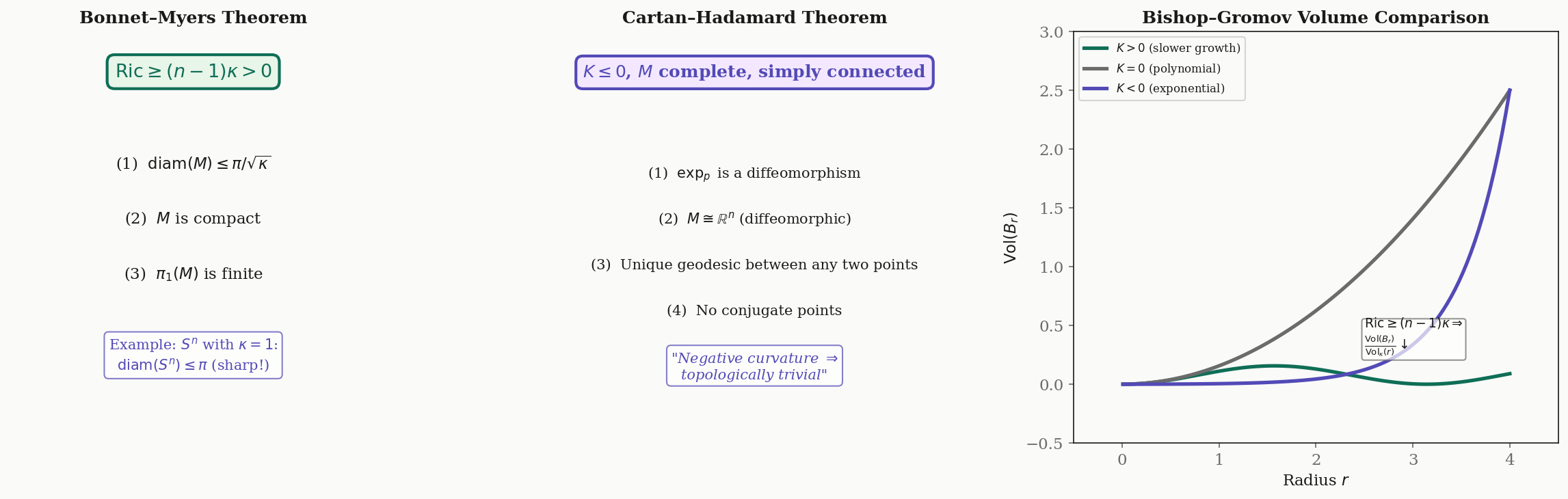
Theorem 8 (Bonnet–Myers Theorem).
Let be a complete Riemannian manifold with Ricci curvature satisfying . Then:
- ,
- is compact,
- is finite (the fundamental group is finite).
The proof uses Jacobi fields: the positive Ricci curvature bound forces geodesics to have conjugate points within distance , so no geodesic can minimize beyond that distance, bounding the diameter. Compactness follows from the Hopf–Rinow theorem. For the unit sphere with , the bound gives , which is sharp.
Theorem 9 (Cartan–Hadamard Theorem).
Let be a complete, simply connected Riemannian manifold with non-positive sectional curvature (). Then:
- is a diffeomorphism (for any ),
- Any two points are connected by a unique geodesic,
- has no conjugate points.
This is the exact opposite of Bonnet–Myers. Non-positive curvature prevents geodesic focusing, so is a global diffeomorphism — the manifold is diffeomorphic to . The topology is completely determined by the curvature sign.
The Rauch comparison theorem makes the relationship between curvature and Jacobi fields precise.
Theorem 10 (Rauch Comparison Theorem).
Let be a geodesic in with sectional curvature along , and let be a geodesic in the space form of constant curvature . Let and be Jacobi fields along and respectively, with and . Then for all before the first conjugate point:
The intuition: more curvature means more focusing, which means shorter Jacobi fields. A manifold with has geodesic deviation bounded above by that of the constant-curvature space .
Theorem 11 (Bishop–Gromov Volume Comparison).
If is a complete Riemannian manifold with , then the ratio
is non-increasing in , where is the volume of a ball of radius in the -dimensional space form of curvature .
The Bishop–Gromov theorem says that positive Ricci curvature constrains volume growth. Geodesic balls in grow no faster than in the model space. This is the foundation of Gromov’s convergence theory and has deep applications in geometric analysis, including the study of Ricci flow (the technique Perelman used to prove the Poincaré conjecture).
Computational Notes
Let’s make the formalism concrete with two computational approaches: symbolic Riemann tensor computation via SymPy, and numerical geodesic solving via SciPy.
Symbolic Riemann tensor for
The following computes the full Riemann tensor, Ricci tensor, and scalar curvature for the sphere of radius using the coordinate formula :
import sympy as sp
from sympy import symbols, sin, cos, diff, trigsimp, Matrix, Rational, latex

theta, phi = symbols('theta phi', positive=True)
r = symbols('r', positive=True)

# Metric tensor: g = r^2 dtheta^2 + r^2 sin^2(theta) dphi^2
g = Matrix([[r**2, 0], [0, r**2 * sin(theta)**2]])
g_inv = g.inv()
coords = [theta, phi]
n = 2

# Christoffel symbols: Gamma^k_ij = (1/2) g^kl (d_j g_li + d_i g_lj - d_l g_ij)
Gamma = [[[0]*n for _ in range(n)] for _ in range(n)]
for k in range(n):
    for i in range(n):
        for j in range(n):
            val = sum(
                Rational(1,2) * g_inv[k,l] * (
                    diff(g[l,i], coords[j]) +
                    diff(g[l,j], coords[i]) -
                    diff(g[i,j], coords[l])
                ) for l in range(n)
            )
            Gamma[k][i][j] = trigsimp(val)

# Riemann tensor: R^l_ijk
R = [[[[0]*n for _ in range(n)] for _ in range(n)] for _ in range(n)]
for l in range(n):
    for i in range(n):
        for j in range(n):
            for k in range(n):
                val = diff(Gamma[l][j][k], coords[i]) - diff(Gamma[l][i][k], coords[j])
                for m in range(n):
                    val += Gamma[l][i][m]*Gamma[m][j][k] - Gamma[l][j][m]*Gamma[m][i][k]
                R[l][i][j][k] = trigsimp(val)
# Result: R^theta_{phi,theta,phi} = sin^2(theta) / r^2 ... (details in notebook)

# Ricci tensor: Ric_ij = R^k_kij
Ric = Matrix(n, n, lambda i,j: trigsimp(sum(R[k][k][i][j] for k in range(n))))
# Result: Ric = diag(1, sin^2(theta))

# Scalar curvature: S = g^ij Ric_ij
S_curv = trigsimp(sum(g_inv[i,j]*Ric[i,j] for i in range(n) for j in range(n)))
# Result: S = 2/r^2, so K = S/2 = 1/r^2 (constant, as expected)
Numerical geodesic solver
The geodesic equation on is a system of 4 first-order ODEs (rewriting the 2 second-order equations):
import numpy as np
from scipy.integrate import solve_ivp

def geodesic_ode(t, y):
    """Geodesic equation on the unit sphere S^2."""
    theta, phi, dtheta, dphi = y
    sin_th, cos_th = np.sin(theta), np.cos(theta)
    # Christoffel symbols: Gamma^theta_{phi,phi} = -sin*cos, Gamma^phi_{theta,phi} = cot
    ddtheta = sin_th * cos_th * dphi**2
    ddphi = -2 * (cos_th / (sin_th + 1e-15)) * dtheta * dphi
    return [dtheta, dphi, ddtheta, ddphi]

# Geodesic from (theta=pi/3, phi=0) in direction (dtheta=0, dphi=1)
y0 = [np.pi/3, 0.0, 0.0, 1.0]
sol = solve_ivp(geodesic_ode, [0, 2*np.pi], y0, max_step=0.01)
# This traces a great circle (latitude circle at theta=pi/3 is NOT a geodesic;
# this initial condition gives a great circle tilted relative to the equator)
Jacobi field magnitude comparison
The closed-form solutions for constant-curvature spaces make the effect of curvature on geodesic deviation concrete:
def jacobi_magnitude(K, t):
    """Jacobi field magnitude for constant sectional curvature K."""
    if abs(K) < 1e-12:
        return t  # flat case
    elif K > 0:
        return np.sin(np.sqrt(K) * t) / np.sqrt(K)
    else:
        return np.sinh(np.sqrt(-K) * t) / np.sqrt(-K)

t = np.linspace(0, 3, 200)
# K=1 (sphere): sin(t) — oscillates, first zero at t=pi (conjugate point)
# K=0 (flat): t — linear growth
# K=-1 (hyperbolic): sinh(t) — exponential growth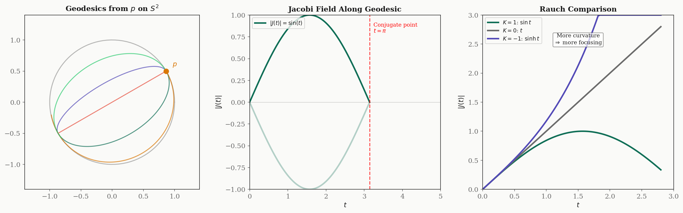
Connections to Machine Learning
Geodesics and curvature are not just abstract geometry — they appear throughout modern machine learning, often in surprising ways.
Manifold learning and reach
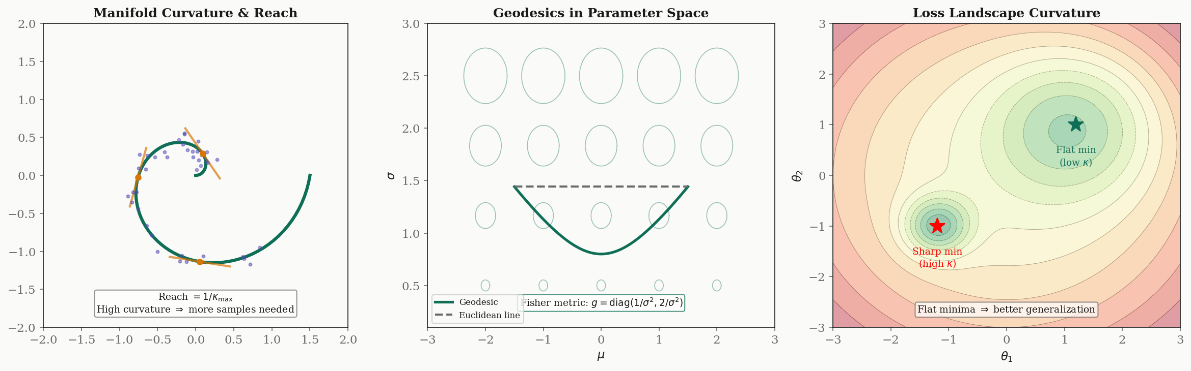
When data lies on a low-dimensional manifold embedded in , the curvature of determines how well local linear approximations (tangent-space PCA) work. The reach of a manifold — roughly, the inverse of the maximum curvature — sets the scale at which the manifold is well-approximated by its tangent planes. Small reach (high curvature) means you need more samples to learn the manifold structure.
Geodesics in parameter space
For a parametric family of distributions , the Fisher information matrix is a Riemannian metric on . Geodesics in the Fisher metric are the “straightest” paths through the parameter space, and they are generally not straight lines in the coordinate .
For the Gaussian family with parameters , the Fisher metric is . The geodesics in this metric are curves in the upper half-plane that locally minimize the Fisher–Rao distance — the intrinsic distance between distributions. Natural gradient descent follows these geodesics rather than the Euclidean straight lines of standard gradient descent.
Loss landscape curvature and generalization
Recent work (Neyshabur et al., 2017; Keskar et al., 2017) connects the curvature of the loss landscape to generalization. The Hessian at a minimum captures the local curvature:
- Flat minima (small Hessian eigenvalues) tend to generalize better — the loss changes slowly in all directions, so the minimum is robust to perturbations.
- Sharp minima (large Hessian eigenvalues) tend to generalize worse — the minimum is sensitive to small changes in parameters.
This is a Riemannian story in disguise: the Hessian plays the role of a curvature tensor on the parameter space, and the “flatness” of a minimum is a statement about the sectional curvatures of the loss surface.
Ollivier–Ricci curvature on graphs
Ollivier (2009) extended the concept of Ricci curvature to discrete metric spaces and graphs. For an edge in a graph, the Ollivier–Ricci curvature compares the Wasserstein distance between probability measures and (random walks from and ) to the graph distance :
Positive curvature () indicates that neighbors of and are closer together than and themselves (community structure). Negative curvature () indicates tree-like or expander-like structure. Ricci flow on graphs — iteratively reweighting edges by their curvature — has been used for community detection and graph simplification.
Connections & Further Reading
Within the Differential Geometry Track
This topic completes the core technical machinery of the Differential Geometry track:
- Smooth Manifolds gave us the differentiable structure — charts, tangent spaces, the differential.
- Riemannian Geometry added the metric tensor, the Levi-Civita connection, and parallel transport.
- Geodesics & Curvature (this topic) builds the geodesic equation, the exponential map, the Riemann tensor and its contractions, the Gauss–Bonnet theorem, Jacobi fields, and the comparison theorems.
Where this leads.
- Information Geometry & Fisher Metric — The Fisher information metric on statistical manifolds makes the parameter space of a model family into a Riemannian manifold. Geodesics in this space give the natural gradient, and the curvature of the statistical manifold determines the local geometry of the KL divergence. This topic provides the complete Riemannian foundation; Information Geometry builds the statistical superstructure.
Connections to Other Tracks
-
The Spectral Theorem — The Ricci tensor at each point is a symmetric bilinear form, and the Spectral Theorem guarantees its diagonalization. The eigenvalues are the principal Ricci curvatures, and the eigenvectors are the directions of maximum and minimum Ricci curvature.
-
Persistent Homology and Simplicial Complexes — The Euler characteristic appearing in the Gauss–Bonnet theorem connects curvature integrals to topological invariants computed by TDA. The alternating sum of Betti numbers equals for a closed surface.
Further Reading
- Lee (2018), Chapters 5–10 — The primary graduate reference for this material. Chapters 5–6 cover geodesics and the exponential map, Chapter 7 covers curvature, and Chapters 8–10 cover Jacobi fields and comparison theorems.
- do Carmo (1992), Chapters 3–8 — A more geometrically oriented treatment with excellent intuition. The Gauss–Bonnet chapter is particularly well-written.
- Cheeger & Ebin (1975) — The definitive reference for comparison theorems, written at a more advanced level.
- Ollivier (2009) — The foundational paper on discrete Ricci curvature for graphs and Markov chains.
Connections
- Geodesics and curvature are the central objects defined by the Riemannian metric and the Levi-Civita connection. The Christoffel symbols from Riemannian Geometry enter directly into the geodesic equation and the Riemann tensor formula. Parallel transport, introduced there, is path-dependent precisely because of curvature. riemannian-geometry
- The manifold structure from Smooth Manifolds — charts, tangent spaces, and the differential — provides the setting for geodesics and curvature. Normal coordinates around a point are a special chart constructed via the exponential map, and the Jacobi equation lives in the tangent bundle. smooth-manifolds
- The Riemann curvature tensor at a point defines a symmetric operator on the space of 2-planes in the tangent space, and its eigenvalues are the principal sectional curvatures. The Spectral Theorem guarantees diagonalization of the Ricci tensor, whose eigenvalues are the principal Ricci curvatures. spectral-theorem
- The Gauss–Bonnet theorem connects Gaussian curvature to the Euler characteristic, which is computed by persistent homology via the alternating sum of Betti numbers. This links the continuous curvature integral to the combinatorial topological invariants of TDA. persistent-homology
- The Euler characteristic chi(M) = V - E + F appearing in the Gauss–Bonnet theorem is computed from any triangulation of the manifold into a simplicial complex, connecting the differential geometry of curvature to the combinatorial topology of simplicial complexes. simplicial-complexes
References & Further Reading
- book Introduction to Riemannian Manifolds — Lee (2018) Chapters 5-10: The primary graduate reference for geodesics, curvature, the exponential map, Jacobi fields, and comparison theorems
- book Riemannian Geometry — do Carmo (1992) Chapters 3-8: Classical treatment of geodesics, curvature, Jacobi fields, and the Gauss–Bonnet theorem with excellent geometric intuition
- book Semi-Riemannian Geometry with Applications to Relativity — O'Neill (1983) Chapters 5-8: Curvature, geodesics, and Jacobi fields in the semi-Riemannian setting with applications to general relativity
- book Comparison Theorems in Riemannian Geometry — Cheeger & Ebin (1975) The definitive reference for Rauch, Bonnet–Myers, Cartan–Hadamard, and Bishop–Gromov comparison theorems
- paper Ricci Curvature of Markov Chains on Metric Spaces — Ollivier (2009) Extends Ricci curvature to discrete metric spaces and Markov chains — the foundation for graph Ricci curvature in ML
- paper Exploring Generalization in Deep Learning — Neyshabur, Bhojanapalli, McAllester & Srebro (2017) Connects loss landscape curvature (sharpness of minima) to generalization bounds in deep learning