Natural Transformations
Morphisms between functors — the naturality condition that distinguishes canonical constructions from arbitrary choices
Overview & Motivation
In Categories & Functors we built the language of categories (objects and morphisms) and functors (structure-preserving maps between categories). We can now ask: what is a morphism between functors?
The answer — a natural transformation — is the concept that Eilenberg and Mac Lane originally invented category theory to define. The term “natural” in mathematics (natural isomorphism, natural map, canonical construction) had been used informally for decades before 1945, when Eilenberg and Mac Lane gave it a precise meaning. A natural transformation is a family of morphisms, one for each object of the source category, that commutes with every morphism in the source. The commutativity condition — the naturality square — is what distinguishes canonical constructions from arbitrary choices.
The central example: every finite-dimensional vector space is isomorphic to its double dual , and this isomorphism is natural — it requires no choice of basis. The embedding is defined uniformly for all , and it commutes with linear maps. By contrast, is also isomorphic to its dual when , but this isomorphism requires choosing a basis — it is not natural.
Why this matters for ML:
- Equivariance is naturality. A CNN’s translation equivariance, a GNN’s permutation equivariance, and a spherical CNN’s rotation equivariance are all instances of the naturality condition. Weight sharing and symmetric aggregation are the mechanisms that enforce naturality.
- The Yoneda lemma — the deepest result we develop here — says that an object is completely determined by its morphisms to all other objects. This is the categorical version of the idea behind distributional semantics, word embeddings, and attention mechanisms: “you shall know a word by the company it keeps.”
- Entropy is natural. Shannon entropy defines a natural transformation from probability distributions to the reals. The data processing inequality — entropy cannot increase under deterministic transformations — is a direct consequence of naturality.
What we cover:
- Natural transformations — the definition, the naturality square, and first examples.
- A gallery of natural transformations — determinant, double dual, abelianization, trace, entropy.
- Composition — vertical, horizontal, whiskering, and the interchange law.
- Functor categories — the category whose objects are functors and whose morphisms are natural transformations.
- The Yoneda lemma — , the deepest result in basic category theory.
- The Yoneda embedding and presheaves — “an object is determined by its relationships.”
- Equivariance as naturality — the categorical perspective on symmetric neural networks.
- Computational notes — verification in Python.
Natural Transformations: Morphisms Between Functors
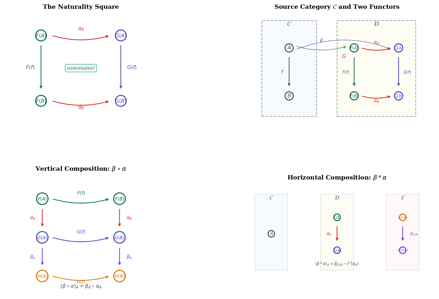
Given two functors between the same pair of categories, a natural transformation is a family of morphisms in — one for each object of — that is “compatible” with the structure of . Compatibility means that for every morphism in , the following square commutes:
The commutativity means . There are two paths from to : go right then down (), or go down then right (). Naturality says both paths give the same morphism.
Definition 1 (Natural Transformation).
Let be functors. A natural transformation is a family of morphisms
called the components of , such that for every morphism in , the naturality condition holds:
We write and denote the set of all natural transformations from to by .
The naturality condition is the key. It says that the transformation is “uniform” across all objects — the component at is determined by the component at in a way that respects the morphism . We can think of this as a consistency condition: if we have two ways of transforming into (via two different paths around the naturality square), they must agree.
Naturality Verification
Double dual: Id ⇒ (-)** in Vec
A Gallery of Natural Transformations
Natural transformations appear everywhere once we know what to look for. Here are the most important examples, starting with the one that motivated the entire theory.
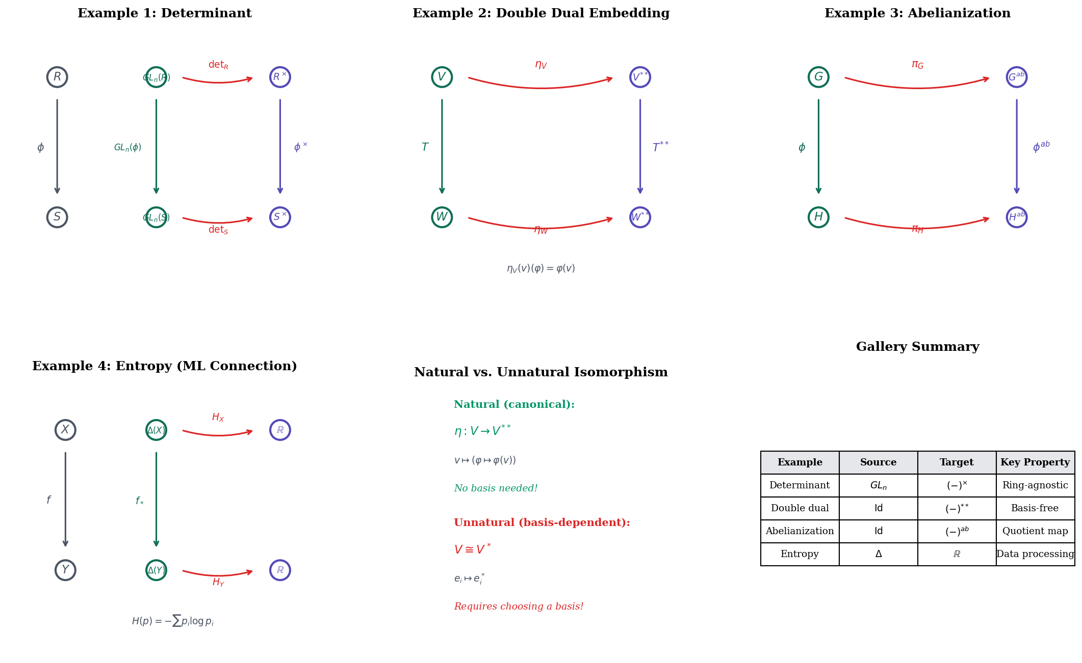
The double dual embedding . For each vector space , the component sends to the evaluation functional defined by . This construction is basis-free — we never chose a basis for . For any linear map , the naturality condition holds: both sides send to the functional on that evaluates at .
The determinant . The functor sends a ring to the group of invertible matrices over , and the functor sends to its group of units . The determinant is a natural transformation: for any ring homomorphism , we have . In words: applying the ring homomorphism entrywise and then taking the determinant gives the same result as taking the determinant first and then applying .
The trace . The functor sends a vector space to its endomorphism ring , and is the constant functor to the ground field. The trace map is natural: for any invertible . Naturality here is the statement that the trace is invariant under change of basis — it depends only on the endomorphism, not on how we represent it.
Abelianization . The functor sends a group to its abelianization . The component is the quotient map. For any group homomorphism , naturality says that abelianizing then mapping is the same as mapping then abelianizing — because sends commutators to commutators.
Entropy as a natural transformation. Shannon entropy defines a natural transformation from the probability distribution functor (which sends a finite set to the set of probability distributions on ) to the constant functor . Naturality says: for any function , , where is the pushforward distribution. This is the data processing inequality — a consequence of naturality.
Remark (Natural vs. Unnatural).
The isomorphism (double dual) is natural — the embedding requires no choice of basis and commutes with linear maps.
The isomorphism (when ) is not natural — every such isomorphism requires choosing a basis (or equivalently, an inner product). Different choices give different isomorphisms, and the construction does not commute with arbitrary linear maps.
The word “natural” in category theory formalizes exactly this distinction: a natural transformation is one that depends only on the structure, not on any choices.
Composition of Natural Transformations
Natural transformations compose in two fundamentally different ways: vertically (stacking transformations end-to-end between functors in a chain ) and horizontally (composing transformations side by side between functor compositions). These two operations interact via the interchange law.
Definition 2 (Vertical Composition).
Given natural transformations and (where ), their vertical composition has components
for each object of .
Proposition 1 (Vertical Composition is Associative).
Vertical composition of natural transformations is associative: for , , .
Proof.
For any object , both sides have component , where the middle equality uses associativity of composition in .
∎Proposition 2 (Identity Natural Transformation).
For each functor , the identity natural transformation with components is a neutral element for vertical composition.
Proof.
For any , and , using the identity law in .
∎Definition 3 (Horizontal Composition).
Given natural transformations (between and ) and (between and ), their horizontal composition has components
The two expressions are equal by the naturality of .
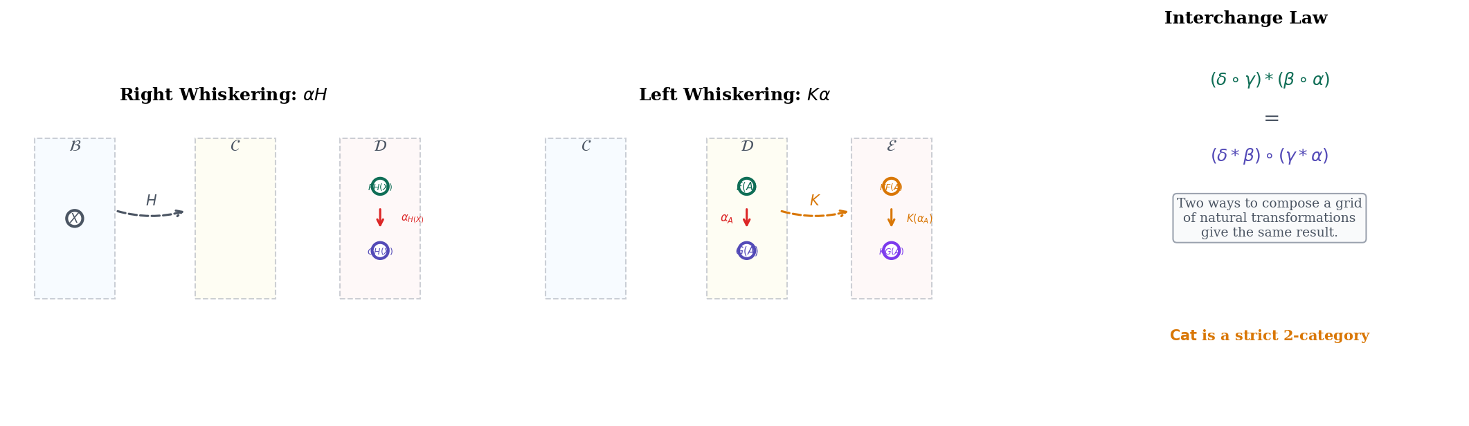
Definition 4 (Whiskering).
Right whiskering: Given (between and ) and a functor , the natural transformation has components .
Left whiskering: Given a functor and (between and ), the natural transformation has components .
Horizontal composition is recovered as .
Proposition 4 (The Interchange Law).
Given natural transformations , (between and ) and , (between and ):
Vertical composition of horizontal composites equals horizontal composition of vertical composites.
Proof.
We compute both sides componentwise at an object of .
Left side: .
Right side: .
These are equal because (functoriality of ) and (naturality of at ). Rearranging using associativity in gives the equality.
∎The interchange law has a deep structural consequence: it gives the 2-category a well-defined notion of “composition of 2-cells” (natural transformations) that is consistent in both directions. This is the starting point of higher category theory.
Functor Categories
Vertical composition with identity natural transformations gives us everything we need to form a category whose objects are functors and whose morphisms are natural transformations.
Definition 5 (Functor Category).
For categories and , the functor category (also written ) is the category whose:
- Objects are functors .
- Morphisms from to are natural transformations .
- Composition is vertical composition of natural transformations.
- Identity on is the identity natural transformation .
Propositions 1 and 2 guarantee that this is indeed a category: vertical composition is associative and identity natural transformations are neutral.
Definition 6 (Natural Isomorphism).
A natural transformation is a natural isomorphism if it is an isomorphism in the functor category — that is, if there exists a natural transformation such that and .
Proposition 3 (Natural Isomorphism iff All Components Invertible).
A natural transformation is a natural isomorphism if and only if every component is an isomorphism in .
Proof.
Forward: If is a natural isomorphism with inverse , then and similarly . So is an isomorphism with inverse .
Backward: Define for each . We must show is natural: that for all . Pre-composing both sides with and post-composing with :
using the naturality of . Since and , the equation gives , and multiplying on the right by gives .
∎Definition 7 (Equivalence of Categories).
An equivalence of categories between and consists of functors and together with natural isomorphisms and .
An equivalence is weaker than an isomorphism of categories (which requires on the nose). Equivalence is the “right” notion of sameness for categories — it says that and have the same categorical structure up to natural isomorphism.
![Functor categories: the category [C,D], identity natural transformation, natural isomorphism, and equivalence of categories](/images/topics/natural-transformations/functor-categories.png)
The Yoneda Lemma
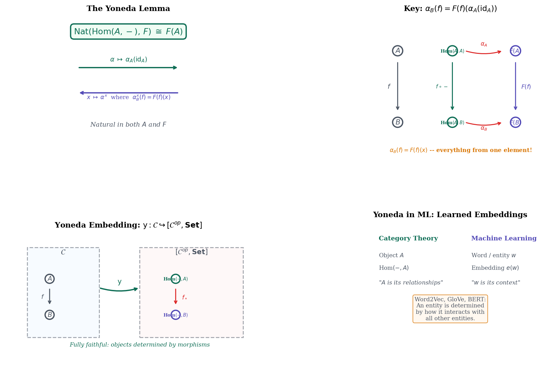
The Yoneda lemma is the deepest result in basic category theory. It says that a natural transformation from a representable functor to any functor is completely determined by a single element of — the image of the identity morphism .
The intuition is this: if we know what does to , then naturality forces the value of on every other morphism. For any , the naturality condition applied to gives:
So where . One element determines everything.
Theorem 1 (The Yoneda Lemma).
Let be a locally small category, a functor, and an object of . There is a bijection
that sends a natural transformation to the element . This bijection is natural in both and .
Proof.
Constructing the bijection. Define . We construct the inverse . Given , define where
for each object and each morphism .
Step 1: is natural. We verify the naturality condition: for ,
These are equal by functoriality of : .
Step 2: . .
Step 3: . Given , let . Then . For any :
where the third equality uses the naturality of at the morphism . So .
Naturality in . Given , the bijection intertwines pre-composition with on the left and on the right: . This is a calculation.
Naturality in . Given a natural transformation , the bijection intertwines post-composition with on the left and on the right: .
∎
The Yoneda Embedding and Presheaves
The Yoneda lemma has an immediate corollary that is one of the most powerful tools in category theory.
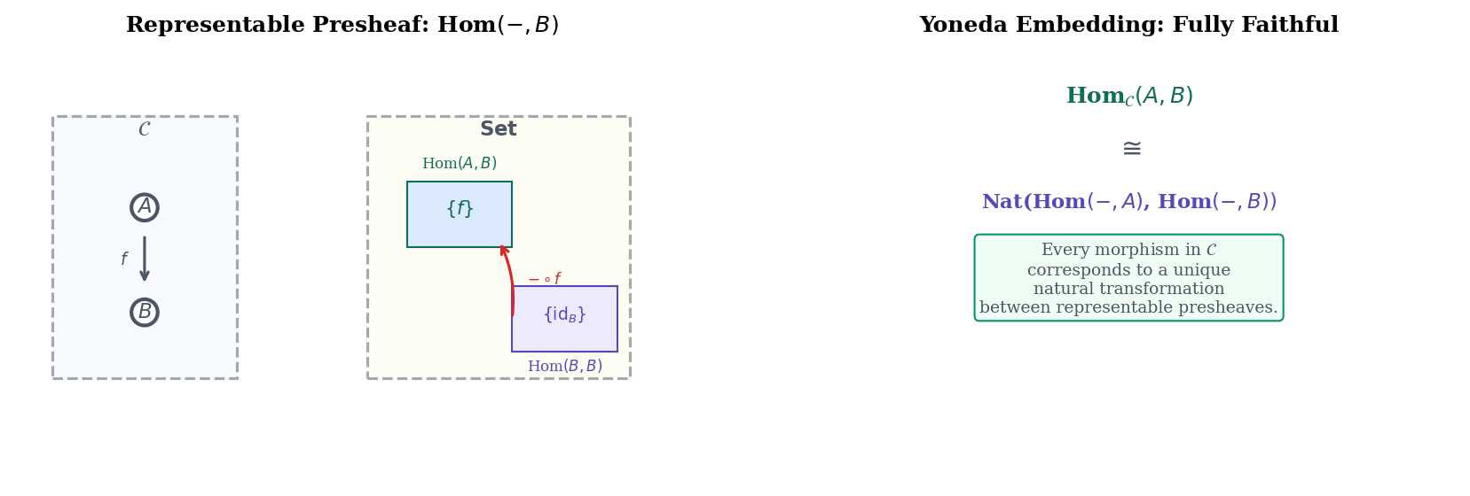
Theorem 2 (The Yoneda Embedding is Fully Faithful).
The Yoneda embedding defined by
is a fully faithful functor. That is, for all objects .
Proof.
Apply the Yoneda lemma with . Then .
∎The Yoneda embedding says: an object is completely determined by its relationships to all other objects. Two objects and are isomorphic if and only if as functors — if and only if they “look the same from the outside.”
Definition 8 (Presheaf).
A presheaf on a category is a functor . The category of presheaves is the functor category , also written .
Definition 9 (Representable Functor).
A presheaf is representable if for some object , called the representing object. By the Yoneda lemma, the representing object is unique up to isomorphism. A natural isomorphism corresponds to a universal element .
Remark (The Yoneda Philosophy in ML).
The Yoneda lemma’s insight — “an object is determined by its morphisms” — appears throughout ML:
-
Distributional semantics and word embeddings. A word is characterized by its co-occurrence patterns with other words. The “distributional hypothesis” is a Yoneda-style principle: two words are semantically similar if they appear in similar contexts, i.e., if their Hom functors are isomorphic.
-
Attention mechanisms. In a transformer, the “value” of a token is determined by its relationships (attention scores) to all other tokens — a computational implementation of the Yoneda perspective.
-
Kernel methods. The kernel trick embeds data points into a reproducing kernel Hilbert space via . This is a Yoneda-like embedding: the point is represented by its similarity function to all other points.
Equivariance as Naturality
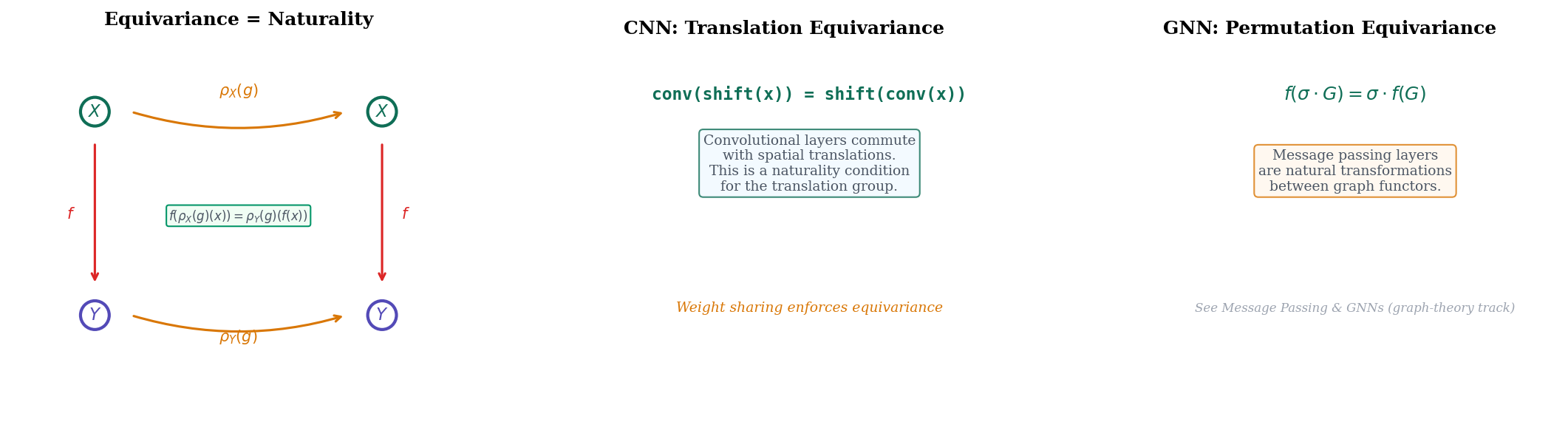
Here is the payoff for readers who have been following both the Category Theory and Graph Theory tracks. The property of equivariance — the requirement that a function commute with a group action — is precisely the naturality condition.
A group defines a one-object category whose single object we call and whose morphisms are the elements of , with composition given by the group operation. A group action of on a set is a functor with and for each .
A function between two -sets is -equivariant if
This is exactly the naturality condition for a natural transformation between the functors ! The naturality square at the morphism is:
Remark (Equivariance as Naturality in Neural Networks).
The three major families of equivariant neural architectures are all instances of naturality:
-
CNNs and translation equivariance. The group is (discrete translations). A convolutional layer commutes with translations because the same filter weights are applied at every position — weight sharing enforces naturality.
-
GNNs and permutation equivariance. The group is (the symmetric group on nodes). A message passing layer commutes with node permutations because aggregation treats all neighbors symmetrically — the aggregation symmetry enforces naturality.
-
Spherical CNNs and rotation equivariance. The group is (3D rotations). Spherical convolutions commute with rotations by design, using harmonic analysis on the sphere.
In each case, the architectural constraint that enforces equivariance is precisely the constraint that makes the layer a natural transformation.
Computational Notes
Here we verify the key examples from this topic in Python, making the abstract mathematics concrete.
Naturality of the double dual embedding. For a linear map , we verify . In finite dimensions with a chosen basis, the double dual embedding is the identity (since canonically), so both paths reduce to :
import numpy as np

T = np.array([[1, 2], [3, 4], [5, 6]])  # T: R^2 -> R^3
v = np.array([1.0, 0.0])

left_path  = T @ v   # T**(eta_V(v)) = T(v) in coordinates
right_path = T @ v   # eta_W(T(v))   = T(v) in coordinates

print(f"Left path  (T** ∘ η_V)(v) = {left_path}")
print(f"Right path (η_W ∘ T)(v)   = {right_path}")
print(f"Naturality holds: {np.allclose(left_path, right_path)}")
The trace as a natural transformation. Naturality means — the trace is invariant under conjugation:
M = np.array([[1.0, 2.0], [3.0, 4.0]])
T_inv = np.array([[0.5, -0.5], [1.0, 0.5]])
T_mat = np.linalg.inv(T_inv)

conjugated = T_mat @ M @ T_inv
print(f"tr(M)          = {np.trace(M):.4f}")
print(f"tr(T M T^(-1)) = {np.trace(conjugated):.4f}")
print(f"Equal: {np.isclose(np.trace(M), np.trace(conjugated))}")
Entropy and the data processing inequality. Shannon entropy defines a natural transformation, and naturality gives us :
from scipy.stats import entropy as scipy_entropy

def entropy_bits(p):
    return scipy_entropy(p, base=2)

def pushforward(p, f_map, target_labels):
    q = {label: 0.0 for label in target_labels}
    for i, pi in enumerate(p):
        q[f_map[i]] += pi
    return np.array([q[label] for label in target_labels])

p = np.array([0.5, 0.3, 0.2])
f_map = {0: "a", 1: "b", 2: "a"}  # f merges elements 0 and 2
f_star_p = pushforward(p, f_map, ["a", "b"])

print(f"H(p)     = {entropy_bits(p):.4f} bits")
print(f"H(f_*p)  = {entropy_bits(f_star_p):.4f} bits")
print(f"H(f_*p) ≤ H(p): {entropy_bits(f_star_p) <= entropy_bits(p) + 1e-10}")
Vertical and horizontal composition. The interchange law can be verified componentwise on small examples. See the companion notebook for full implementations.
Connections & Further Reading
Where this fits
Natural transformations are the second topic in the Category Theory track and the conceptual bridge between the static structure of categories/functors and the dynamic structure of adjunctions and monads:
-
Categories & Functors — the direct prerequisite. All definitions (categories, functors, morphisms, composition, Hom sets, opposite categories) are assumed.
-
Adjunctions — formalizes the unit-counit pairs as natural transformations satisfying the triangle identities, with the free-forgetful paradigm as the primary example. The Hom-set definition requires naturality in both variables, and the Yoneda lemma underlies the uniqueness-of-adjoints proof.
-
Monads & Comonads — uses natural transformations as the defining data: the unit and multiplication are natural transformations whose commutative diagrams encode the monad laws. A monad is a monoid in the functor category — whose morphisms are natural transformations.
Cross-track connections
-
Shannon Entropy & Mutual Information — entropy as a natural transformation from the probability distribution functor to the reals; the data processing inequality as a consequence of naturality.
-
Message Passing & GNNs — permutation equivariance of message passing layers is precisely the naturality condition for the symmetric group action on node features.
-
The Spectral Theorem — the double dual embedding and the trace are natural transformations in Vec, the category where the spectral theorem lives.
-
Measure-Theoretic Probability — the Dirac delta embedding is a natural transformation from the identity functor to the probability measure functor, forming the unit of the Giry monad.
-
Smooth Manifolds — the de Rham theorem establishes a natural isomorphism between de Rham cohomology and singular cohomology.
Notation summary
| Symbol | Meaning |
|---|---|
| Natural transformation from to | |
| Component of at object | |
| Vertical composition | |
| Horizontal composition | |
| Right whiskering (pre-compose with ) | |
| Left whiskering (post-compose with ) | |
| Set of natural transformations from to | |
| Functor category | |
| Natural isomorphism | |
| Yoneda embedding | |
| Covariant representable functor | |
| Contravariant representable functor | |
| Presheaf category | |
| Double dual of | |
| Group action of on | |
| One-object category associated to group | |
| Unit of a monad (preview) |
Connections
- Direct prerequisite. All definitions — categories, functors, morphisms, composition, identity, Hom sets, opposite categories — are assumed. The Hom functor and its covariant/contravariant versions, introduced in Topic 1, are central to the Yoneda lemma. categories-functors
- Shannon entropy H defines a natural transformation from the probability distribution functor Delta to the constant functor R. The data processing inequality — H(f_*(p)) <= H(p) for deterministic functions f — is a consequence of the naturality of entropy. shannon-entropy
- Message passing layers in graph neural networks are natural transformations between graph functors. Permutation equivariance of GNNs — f(sigma . G) = sigma . f(G) — is precisely the naturality condition for the symmetric group action. message-passing
- The double dual embedding eta_V: V -> V** is a natural transformation Id => (-)** in Vec. The trace tr: End(-) -> k is a natural transformation from the endomorphism functor to the ground field. Both are canonical (basis-independent) constructions. spectral-theorem
- The Giry monad's unit (Dirac delta embedding delta: X -> P(X)) is a natural transformation Id => P. Conditioning and marginalization are natural transformations between probability functors on Meas. measure-theoretic-probability
- The de Rham theorem establishes a natural isomorphism between de Rham cohomology and singular cohomology. Naturality ensures that pullbacks of differential forms commute with the cohomology isomorphism. smooth-manifolds
References & Further Reading
- book Categories for the Working Mathematician — Mac Lane (1998) Chapters IV-V cover natural transformations, the Yoneda lemma, and functor categories — the definitive treatment
- book Category Theory — Awodey (2010) Chapter 7 on natural transformations with accessible examples from algebra
- book Category Theory in Context — Riehl (2016) Chapters 2-3 develop natural transformations and the Yoneda lemma in depth — freely available online
- book An Invitation to Applied Category Theory: Seven Sketches in Compositionality — Fong & Spivak (2019) Applied examples of naturality in databases, circuits, and ML pipelines
- paper Category Theory in Machine Learning — Shiebler, Gavranović & Wilson (2021) Sections on equivariant neural networks as natural transformations and categorical probability
- paper Geometric Deep Learning: Grids, Groups, Graphs, Geodesics, and Gauges — Bronstein, Bruna, Cohen, & Veličković (2021) Equivariance as a unifying design principle for neural architectures — the group-theoretic perspective that naturality formalizes