Message Passing & GNNs
From spectral graph convolutions to neighborhood aggregation — the mathematical foundations of graph neural networks
Overview & Motivation
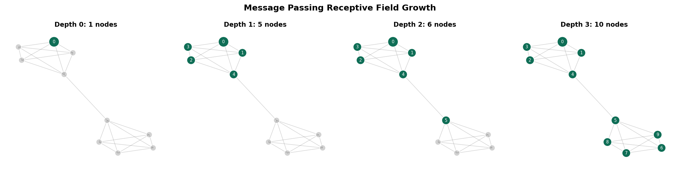
A graph neural network learns representations by passing messages along edges. At each layer, every node aggregates information from its neighbors, transforms the result, and produces an updated feature vector. After layers, each node’s representation encodes the structure of its -hop neighborhood.
This idea unifies the entire Graph Theory track:
- Graph Laplacians: The GCN update rule is one step of Laplacian smoothing on the renormalized graph. The filter is a first-order polynomial of the normalized Laplacian.
- Random Walks: Repeated message passing drives node features toward the stationary distribution . The spectral gap controls how many layers before features become indistinguishable — the over-smoothing phenomenon.
- Expander Graphs: On expanders, information reaches all nodes in layers — optimal receptive field growth. But over-smoothing also occurs in layers. Expander-based rewiring adds long-range edges to bottlenecked graphs, importing the expansion benefits without the over-smoothing cost.
What this topic covers:
- The message passing framework — aggregate, update, readout as the universal GNN template.
- Spectral graph convolutions — from the graph Fourier transform to ChebNet to GCN as Laplacian smoothing.
- Spatial graph convolutions — GCN, GraphSAGE, GIN, and the neighborhood aggregation perspective.
- The Weisfeiler-Leman test — 1-WL isomorphism test, equivalence to message passing GNNs, and the expressiveness hierarchy.
- Attention-based message passing — Graph Attention Networks (GAT) and learned edge weights.
- Over-smoothing — the random walk convergence connection, Dirichlet energy decay, and depth limitations.
- Expander-based graph rewiring — SDRF, FoSR, and spectral gap optimization as architectural design.
The Message Passing Framework
The message passing neural network (MPNN) framework unifies virtually all graph neural network architectures into three phases: aggregate, update, and readout. We develop each in turn.
The MPNN Template
Definition (Definition 1 — Message Passing Neural Network (MPNN)).
A message passing neural network operates on a graph with node features . At each layer , two operations transform the features:
where is a permutation-invariant aggregation (sum, mean, max), is the message function, is the update function, and encodes optional edge features.
For graph-level tasks, a readout function pools all node representations:
Matrix Form
For simple message passing (linear messages, mean aggregation), the layer update collapses to a matrix equation. Let collect node features as rows:
where is a normalized adjacency operator and is the learnable weight matrix. Different choices of yield different architectures:
| Architecture | Name | |
|---|---|---|
| GCN (Kipf & Welling) | Renormalized symmetric | |
| GraphSAGE (mean) | Transition matrix | |
| Simple GCN | Normalized adjacency (no self-loops) |
Receptive Field Growth
After layers of message passing, each node’s representation depends on all nodes within hops. The receptive field of node at depth is the -hop neighborhood .
Proposition (Proposition 1 — Receptive Field and Diameter).
For a connected graph with diameter , layers suffice for every node to receive information from every other node.
On expander graphs, , so logarithmic depth is sufficient. On path graphs, , requiring linear depth.
Spectral Graph Convolutions
The spectral perspective interprets message passing through the lens of the graph Laplacian eigendecomposition.
The Graph Fourier Transform
Definition (Definition 2 — Graph Fourier Transform).
Given the normalized Laplacian with orthonormal eigenvectors and eigenvalues , the graph Fourier transform of a signal is:
The inverse transform recovers the signal: .
The eigenvectors play the role of Fourier modes: (the constant vector) is the “DC component,” and higher eigenvectors oscillate more across the graph. The eigenvalue measures the frequency — low means smooth variation along edges, high means rapid oscillation.
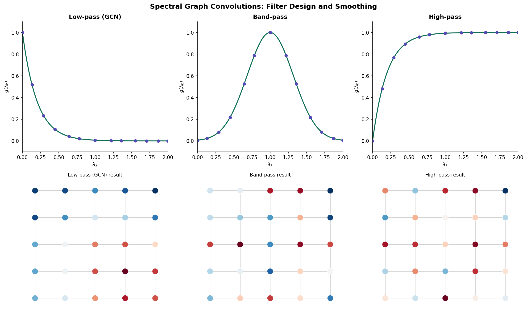
Spectral Convolution
Definition (Definition 3 — Spectral Graph Convolution).
A spectral graph convolution applies a filter in the Fourier domain:
where is the spectral transfer function.
The problem: learning free parameters is expensive and non-transferable (different graphs have different eigenvectors).
ChebNet and Polynomial Filters
Theorem (Theorem 1 — Chebyshev Approximation (Defferrard, Bresson & Vandergheynst 2016)).
Approximating with a -th order Chebyshev polynomial:
where and is the -th Chebyshev polynomial, yields a -localized filter that depends only on -hop neighborhoods. The convolution becomes:
This avoids the eigenvector computation entirely — is computed via the Chebyshev recurrence applied to the matrix.
GCN as a First-Order Spectral Filter
Theorem (Theorem 2 — GCN is First-Order Spectral (Kipf & Welling 2017)).
Setting and in the ChebNet filter yields:
Constraining to reduce parameters:
The renormalization trick replaces with where and , yielding the GCN layer:
Proof. The eigenvalues of lie in , which causes numerical instabilities under repeated application. Adding self-loops via shifts the spectrum: if is an eigenvalue of , the corresponding eigenvalue of is approximately . This keeps eigenvalues bounded and prevents gradient explosion under deep stacking.
Remark (Remark — GCN is Laplacian Smoothing).
Applying to node features is equivalent to replacing each node’s features with a weighted average of its own features and its neighbors’. This is a low-pass filter on the graph — it suppresses high-frequency components (large ) and preserves low-frequency structure (small ). This connection to the Laplacian spectrum is why GCN smooths features and why deep GCNs over-smooth.
Spatial Graph Convolutions
The spatial perspective bypasses eigendecomposition entirely. Instead of filtering in the spectral domain, we directly define how each node aggregates neighbor features.
GCN (Kipf & Welling 2017)
The GCN layer with mean aggregation:
This is equivalent to the spectral derivation via the renormalized adjacency.
GraphSAGE (Hamilton, Ying & Leskovec 2017)
GraphSAGE separates the self-loop from neighbor aggregation:
where AGG can be mean, LSTM, or max-pool. The concatenation preserves the node’s own identity separately from its aggregated neighborhood.
GIN (Xu, Hu, Leskovec & Jegelka 2019)
Definition (Definition 4 — Graph Isomorphism Network (GIN)).
The GIN update uses sum aggregation with a learnable self-loop weight :
GIN is the most expressive architecture within the MPNN framework — it is exactly as powerful as the 1-WL isomorphism test.
The Weisfeiler-Leman Test & GNN Expressiveness
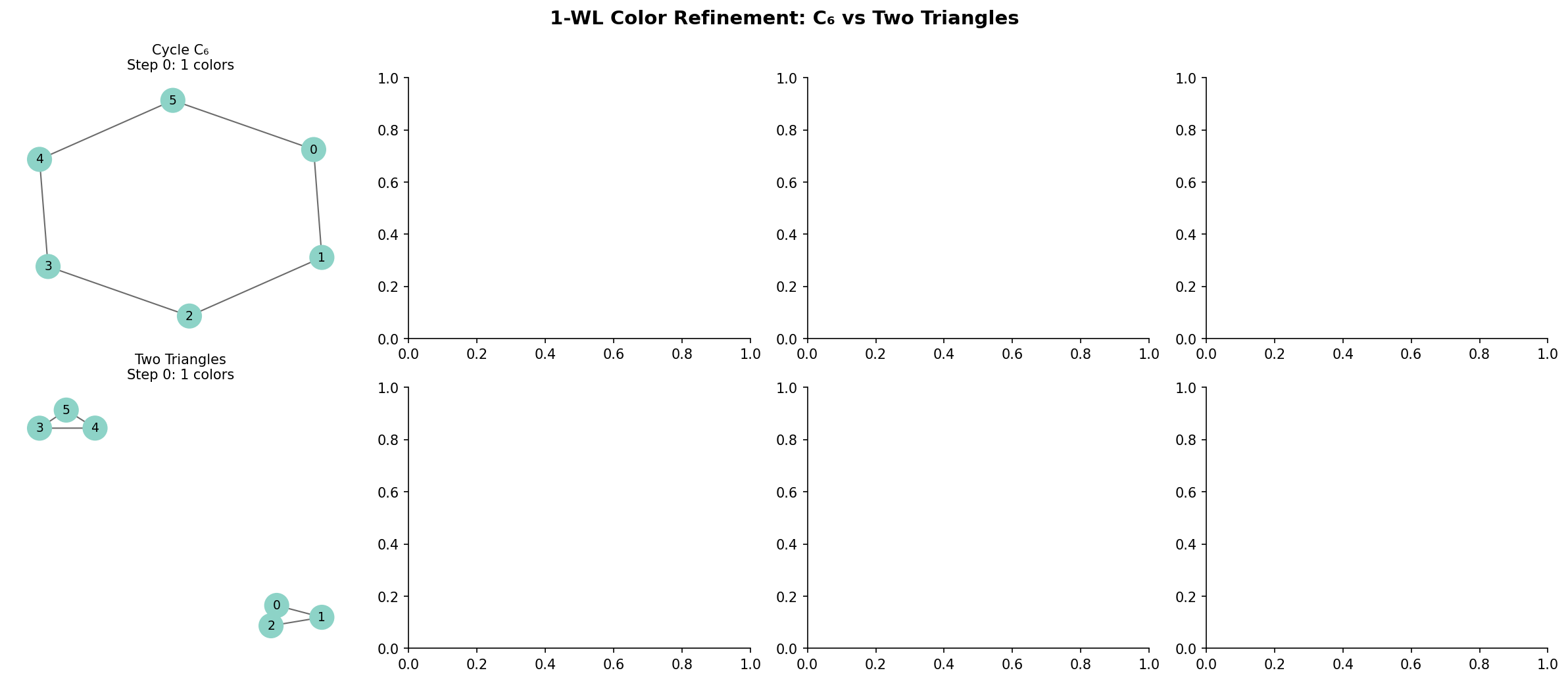
The 1-WL Color Refinement Algorithm
Definition (Definition 5 — 1-WL Color Refinement).
The 1-dimensional Weisfeiler-Leman test is an iterative color refinement algorithm for testing graph isomorphism:
- Initialize: assign each node a color (typically based on degree or a constant).
- Refine: update colors by hashing the multiset of neighbor colors:
- Halt: when the color partition stabilizes (no further refinement).
- Decide: if the multiset of final colors differs between two graphs, they are not isomorphic. If they agree, the test is inconclusive.
GNN = 1-WL (in Expressive Power)
Theorem (Theorem 3 — MPNN ≤ 1-WL Expressiveness (Xu, Hu, Leskovec & Jegelka 2019)).
A message passing GNN is at most as expressive as the 1-WL test: if 1-WL cannot distinguish two graphs and , then no MPNN can produce different representations for them.
Proof sketch. The MPNN update maps the multiset of neighbor features through a permutation-invariant aggregation . If two nodes in and in have the same 1-WL color at step , they have the same multiset of neighbor colors, so any aggregation produces the same result. By induction, MPNNs cannot distinguish what 1-WL cannot.
Theorem (Theorem 4 — GIN Matches 1-WL).
With injective aggregation (sum) and a sufficiently expressive update function (MLP), GIN achieves 1-WL expressiveness: it can distinguish any pair of graphs that 1-WL distinguishes.
Proof sketch. Sum aggregation over a multiset is injective if composed with a universal function approximator (the MLP). The hash function in 1-WL is injective on multisets, and the MLP can approximate it arbitrarily well. Therefore, GIN simulates 1-WL exactly.
Limitations of 1-WL
Remark (Remark — Regular Graphs and 1-WL Failure).
The 1-WL test cannot distinguish all non-isomorphic regular graphs. For example, the Rook’s graph and the Paley graph of order 9 are both 4-regular on 9 vertices but not isomorphic — yet 1-WL assigns them identical color histograms. No standard MPNN can distinguish them either.
Higher-order WL tests (-WL for ) can distinguish more graphs by operating on -tuples of vertices rather than individual vertices. -WL GNNs are correspondingly more expressive but have complexity.
Attention-Based Message Passing
Graph Attention Networks (GAT)
Definition (Definition 6 — Graph Attention Layer (GAT — Veličković et al. 2018)).
The GAT layer computes attention coefficients between connected nodes:
where is a learnable attention vector, is a shared weight matrix, and denotes concatenation.
Theorem (Theorem 5 — GAT Generalizes GCN).
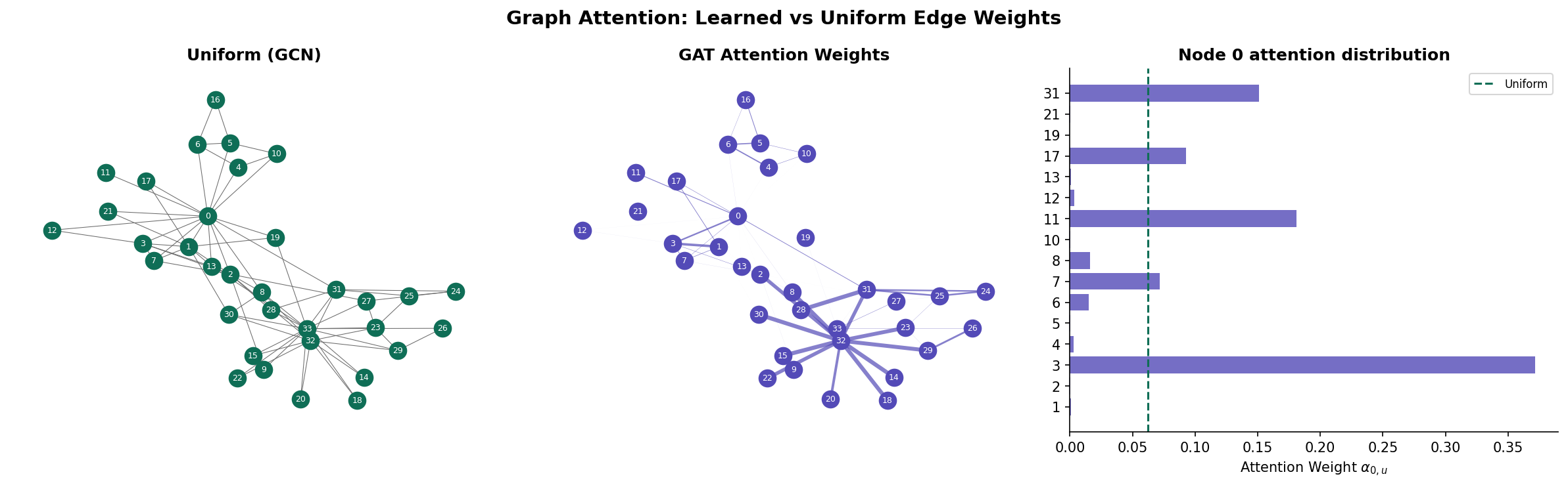
When attention weights are set to (inverse-degree normalization), the GAT layer reduces to the GCN layer. GCN is therefore GAT with uniform, structure-dependent attention.
Proof. In GCN, the entry of is for adjacent (including self-loops). Setting to this constant (independent of features) recovers the GCN update exactly. GAT generalizes this by making depend on node features, allowing the model to learn which neighbors are more relevant.
Multi-Head Attention
GAT uses multi-head attention to stabilize training:
where denotes concatenation over attention heads. Each head learns different edge importance patterns.
The Attention Matrix Perspective
The attention weights define a learned, data-dependent graph: the attention graph where edge has weight . This is a soft version of graph rewiring — attention can effectively increase or decrease edge weights, reshaping the message-passing topology without changing the underlying graph.
Over-Smoothing & the Random Walk Connection
The Over-Smoothing Problem
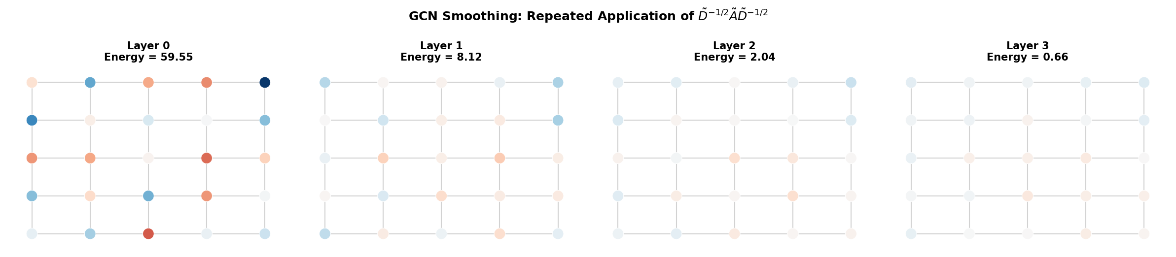
Definition (Definition 7 — Over-Smoothing (Dirichlet Energy)).
A GNN suffers from over-smoothing when repeated message passing drives all node representations toward the same value, destroying the discriminative power needed for node-level tasks.
The Dirichlet energy of node features on a graph with Laplacian :
Over-smoothing occurs when as .
Over-Smoothing is Random Walk Convergence
Theorem (Theorem 6 — Over-Smoothing Rate (Li, Han & Wu 2018)).
For a GCN without nonlinearity () and identity weights (), the feature matrix after layers is:
where . Since is a stochastic-like matrix with spectral radius 1, repeated application converges to the rank-1 projection:
where is the eigenvector corresponding to eigenvalue 1.
Proof. By the spectral decomposition, where . Then since for . The rate of convergence is , and the spectral gap of the random walk is .
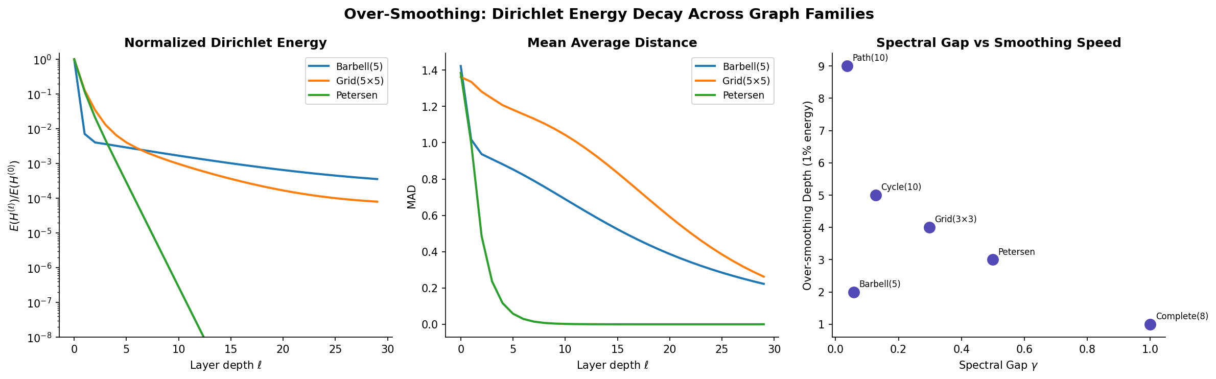
The Dirichlet energy decays as .
Corollary (Corollary 1 — Over-Smoothing on Expanders).
On an -expander, the Dirichlet energy decays exponentially with rate . Over-smoothing occurs in layers — the same depth that provides the optimal receptive field. Expansion is a double-edged sword: it enables rapid information propagation but equally rapid feature homogenization.
Measuring Over-Smoothing: MAD and Dirichlet Energy
Definition (Definition 8 — Mean Average Distance (MAD — Chen et al. 2020)).
The Mean Average Distance of node features measures representational diversity:
indicates complete over-smoothing. A healthy GNN maintains across layers.
Mitigation Strategies
Several strategies combat over-smoothing:
- Residual connections: preserves the original signal.
- Jumping knowledge: accesses all depths.
- DropEdge: Randomly remove edges during training to slow diffusion.
- PairNorm / NodeNorm: Normalize features to maintain diversity.
- Graph rewiring: Add long-range edges to reduce diameter without adding layers (see next section).
Expander-Based Graph Rewiring
The Bottleneck Problem
Many real-world graphs have bottlenecks — vertices or small edge cuts that separate communities. From the Cheeger inequality, a small spectral gap implies a tight bottleneck . Message passing across the bottleneck requires layers — far more than the receptive field within each community.
Graph Rewiring via Spectral Gap Optimization
Definition (Definition 9 — Spectral Gap Rewiring).
Graph rewiring adds “shortcut” edges to increase the spectral gap without changing the original node features. The rewired graph has:
- All original edges of
- Additional edges chosen to maximize
Proposition (Proposition 2 — SDRF (Topping et al. 2022)).
The Stochastic Discrete Ricci Flow (SDRF) rewiring algorithm iteratively adds edges between vertices with negative Ricci curvature (bottleneck regions) and removes edges with high curvature (redundant connections). After rewiring steps, SDRF provably increases the spectral gap.
Expander Graph Augmentation
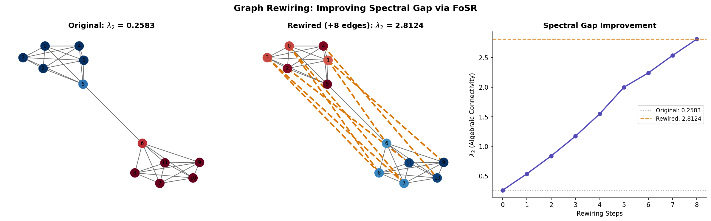
Theorem (Theorem 7 — FoSR Spectral Gap Improvement (Deac et al. 2022)).
First-Order Spectral Rewiring (FoSR) adds edges that approximately maximize the increase in using the Fiedler vector. At each step, it adds the edge maximizing where is the Fiedler vector. After rewiring steps, the spectral gap satisfies:
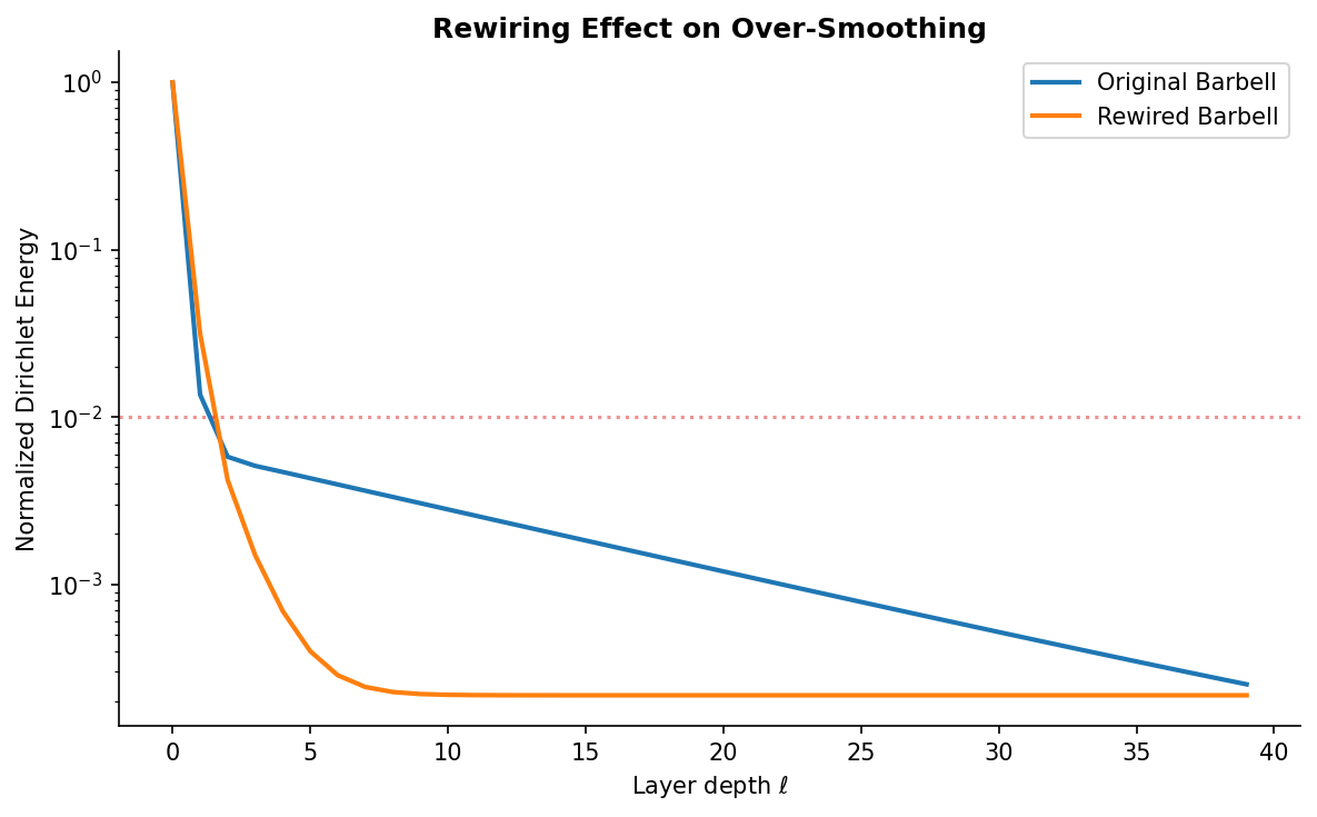
Remark (Remark — Connection to Expanders).
The goal of spectral rewiring is to make the graph “more expander-like” — increasing moves the graph toward the Ramanujan bound . A fully rewired graph with gives:
- receptive field (from expansion)
- over-smoothing depth (the tradeoff)
- But the added edges carry no original features — they only accelerate diffusion
Beyond Standard Message Passing
Several architectures break the message passing paradigm to overcome its limitations:
| Architecture | Key Innovation | Expressiveness |
|---|---|---|
| Graph Transformers | Full self-attention (no edge constraint) | Beyond 1-WL |
| k-GNN | Higher-order WL (k-tuples) | -WL |
| Subgraph GNNs | Run MPNN on subgraph ensembles | 3-WL |
| Equivariant GNNs | Geometric symmetries (E(3), SE(3)) | Task-dependent |
Computational Notes
PyTorch Geometric
The standard library for GNN implementation in Python is PyTorch Geometric (PyG). A GCN layer in PyG:
import torch
from torch_geometric.nn import GCNConv

class GCN(torch.nn.Module):
    def __init__(self, in_channels, hidden_channels, out_channels):
        super().__init__()
        self.conv1 = GCNConv(in_channels, hidden_channels)
        self.conv2 = GCNConv(hidden_channels, out_channels)

    def forward(self, x, edge_index):
        x = self.conv1(x, edge_index).relu()
        x = self.conv2(x, edge_index)
        return x
DGL (Deep Graph Library)
An alternative implementation framework:
import dgl
import torch
from dgl.nn import GraphConv

class GCN(torch.nn.Module):
    def __init__(self, in_feats, h_feats, num_classes):
        super().__init__()
        self.conv1 = GraphConv(in_feats, h_feats)
        self.conv2 = GraphConv(h_feats, num_classes)

    def forward(self, g, in_feat):
        h = self.conv1(g, in_feat).relu()
        h = self.conv2(g, h)
        return h
Spectral vs Spatial Complexity
| Approach | Per-Layer Cost | Localized? | Transferable? |
|---|---|---|---|
| Full spectral () | No | No | |
| ChebNet (order ) | -hop | Yes | |
| GCN (1st order) | 1-hop | Yes | |
| GAT | 1-hop | Yes | |
| Graph Transformer | Global | Yes |
Monitoring Over-Smoothing
Track Dirichlet energy and MAD during training to detect over-smoothing:
def dirichlet_energy_torch(x, edge_index):
    row, col = edge_index
    diff = x[row] - x[col]
    return (diff ** 2).sum()
If energy drops below a threshold after the first few layers, consider reducing depth, adding residual connections, or applying graph rewiring.
Connections & Further Reading
Cross-Track and Within-Track Connections
| Topic | Track | Connection |
|---|---|---|
| Graph Laplacians & Spectrum | Graph Theory | The GCN update rule is a first-order polynomial of the normalized Laplacian. Spectral graph convolutions filter signals via the Laplacian eigendecomposition. The Fiedler vector drives spectral rewiring. |
| Random Walks & Mixing | Graph Theory | Over-smoothing is random walk convergence: repeated application of drives features to the stationary distribution. The spectral gap controls the over-smoothing rate. Mixing time bounds directly predict GNN depth limits. |
| Expander Graphs | Graph Theory | Expanders give receptive fields but also over-smoothing depth. Expander-based graph rewiring (FoSR, SDRF) increases to improve information flow. The Expander Mixing Lemma implies quasi-random message passing on expanders. |
| The Spectral Theorem | Linear Algebra | The spectral decomposition of underlies both GCN smoothing analysis and the 1-WL expressiveness proof. Eigenvalue bounds govern convergence rates. |
| Gradient Descent & Convergence | Optimization | GNNs are trained via backpropagation through message-passing layers. The gradient flow through suffers from vanishing/exploding gradients governed by the spectral radius. |
| PCA & Low-Rank Approximation | Linear Algebra | Node embeddings from GNNs approximate a low-rank factorization of the graph. DeepWalk = implicit matrix factorization. Spectral clustering uses the bottom Laplacian eigenvectors as a low-rank embedding. |
| Concentration Inequalities | Probability & Statistics | PAC-style generalization bounds for GNNs use Rademacher complexity. The number of message-passing layers affects the model’s effective capacity and generalization. |
Notation Summary
| Symbol | Meaning |
|---|---|
| Node ‘s feature vector at layer | |
| Feature matrix at layer () | |
| Learnable weight matrix at layer | |
| Normalized adjacency operator (GCN: ) | |
| Permutation-invariant aggregation (sum, mean, max) | |
| GAT attention weight from to | |
| Dirichlet energy: | |
| 1-WL color of node at iteration | |
| Mean Average Distance of node features |
Connections
- The GCN update rule is a first-order polynomial of the normalized Laplacian: spectral graph convolutions filter signals via the Laplacian eigendecomposition. The Fiedler vector drives spectral rewiring (FoSR), and Cheeger's inequality bounds the information bottleneck that limits message passing depth. graph-laplacians
- Over-smoothing is random walk convergence: repeated application of the normalized adjacency drives features to the stationary distribution π. The spectral gap γ = 1 − λ₂(P) controls the over-smoothing rate, and the mixing time bounds from random walk theory directly predict GNN depth limits. random-walks
- Expanders give O(log n) receptive fields but also O(log n) over-smoothing depth — the fundamental tradeoff. Expander-based rewiring (FoSR, SDRF) increases λ₂ to improve information flow. The Expander Mixing Lemma implies quasi-random message passing on expanders. expander-graphs
- The spectral decomposition of the normalized adjacency underlies both the GCN smoothing analysis and the over-smoothing convergence proof. The eigenvectors form the graph Fourier basis, and eigenvalue bounds govern the convergence rate of iterated message passing. spectral-theorem
- GNNs are trained via backpropagation through L layers of message passing. The gradient flows through Â^L, where vanishing/exploding gradient behavior is governed by the spectral radius — the same convergence analysis from gradient descent theory. gradient-descent
- Node embeddings from GNNs approximate a low-rank factorization of the graph. DeepWalk is implicit matrix factorization (Qiu et al. 2018). Spectral clustering uses the bottom Laplacian eigenvectors as a low-rank embedding — the non-parametric precursor to learned graph embeddings. pca-low-rank
- PAC-style generalization bounds for GNNs use Rademacher complexity and VC dimension. The number of message-passing layers affects the model's effective capacity, and concentration inequalities bound the gap between training and test performance. concentration-inequalities
References & Further Reading
- paper Semi-Supervised Classification with Graph Convolutional Networks — Kipf & Welling (2017) The GCN paper — spectral derivation, renormalization trick, and the architecture that launched graph deep learning
- paper Neural Message Passing for Quantum Chemistry — Gilmer, Schoenholz, Riley, Vinyals & Dahl (2017) The MPNN framework that unifies GNN architectures into aggregate-update-readout
- paper How Powerful are Graph Neural Networks? — Xu, Hu, Leskovec & Jegelka (2019) GIN paper — proves MPNN ≤ 1-WL expressiveness and shows GIN matches 1-WL
- paper Graph Attention Networks — Veličković, Cucurull, Casanova, Romero, Liò & Bengio (2018) GAT — learned attention-based aggregation replacing uniform neighborhood weights
- paper Deeper Insights into Graph Convolutional Networks for Semi-Supervised Learning — Li, Han & Wu (2018) Over-smoothing analysis — proves GCN is Laplacian smoothing and characterizes depth limits
- paper Understanding Over-Squashing and Bottlenecks on Graphs via Curvature — Topping, Di Giovanni, Chamberlain, Dong & Bronstein (2022) SDRF rewiring — discrete Ricci curvature identifies bottlenecks and guides edge addition
- paper Expander Graph Propagation — Deac, Lackenby & Veličković (2022) FoSR — first-order spectral rewiring using the Fiedler vector to maximize λ₂
- paper Convolutional Neural Networks on Graphs with Fast Localized Spectral Filtering — Defferrard, Bresson & Vandergheynst (2016) ChebNet — Chebyshev polynomial spectral filters, the precursor to GCN
- paper Weisfeiler and Leman Go Neural: Higher-Order Graph Neural Networks — Morris, Ritzert, Fey, Hamilton, Lenssen, Rattan & Grohe (2019) k-WL GNNs — higher-order expressiveness beyond standard message passing