Concentration Inequalities

Overview & Motivation

The Measure-Theoretic Probability topic established that sample averages converge to population means. The Weak Law of Large Numbers tells us $\bar{X}_n \xrightarrow{P} \mu$. The Strong Law strengthens this to almost sure convergence. But neither law answers the question a practitioner actually asks: how many samples do we need?

Suppose we train a classifier on $n$ samples and observe an empirical error rate of 5%. How confident are we that the true error is close to 5%? The law of large numbers says “eventually” — but “eventually” is not a sample size. We need quantitative bounds on tail probabilities: explicit formulas relating $n$, the error tolerance $\varepsilon$, and the failure probability $\delta$.

This is exactly what concentration inequalities provide. They answer questions of the form:

$P\left(|\bar{X}_n - \mu| \geq \varepsilon\right) \leq f(n, \varepsilon)$

where $f$ decreases (typically exponentially) in $n$ and $\varepsilon$. Inverting these bounds gives us sample complexity: the number of samples sufficient to guarantee $|\bar{X}_n - \mu| < \varepsilon$ with probability at least $1 - \delta$.

The progression of tightness. We develop a hierarchy of increasingly powerful bounds:

1. Markov’s inequality uses only the mean — the weakest bound but the most general.
2. Chebyshev’s inequality adds the variance — a polynomial ($1/n$) rate.
3. Chernoff bounds exploit the full moment generating function — exponential ($e^{-cn}$) rates.
4. Hoeffding’s inequality provides a clean, usable exponential bound for bounded random variables.
5. Sub-Gaussian theory abstracts the pattern: a random variable concentrates like a Gaussian if its MGF is controlled by a quadratic.
6. Bernstein’s inequality refines the bound when the variance is small relative to the range.
7. McDiarmid’s inequality extends concentration from sums to arbitrary functions of independent variables.

Each step trades generality for tightness. By the end, we will have the precise tools to prove generalization bounds — the theoretical guarantee that a machine learning model’s training error approximates its true error — and derive sample complexity results for finite hypothesis classes.

---

Basic Tail Bounds: Markov and Chebyshev

The Tail Probability Question

Given a random variable $X$ with known moments (mean, variance, etc.), what can we say about the probability that $X$ deviates far from its expected value? This is the tail probability question, and it is the foundation of all concentration inequalities.

We begin with the simplest possible bound, which uses only the first moment.

Markov’s Inequality

Chebyshev’s Inequality

We can obtain a tighter bound by exploiting the variance. The idea is simple: apply Markov’s inequality to $|X - \mu|^2$.

One-Sided Variants

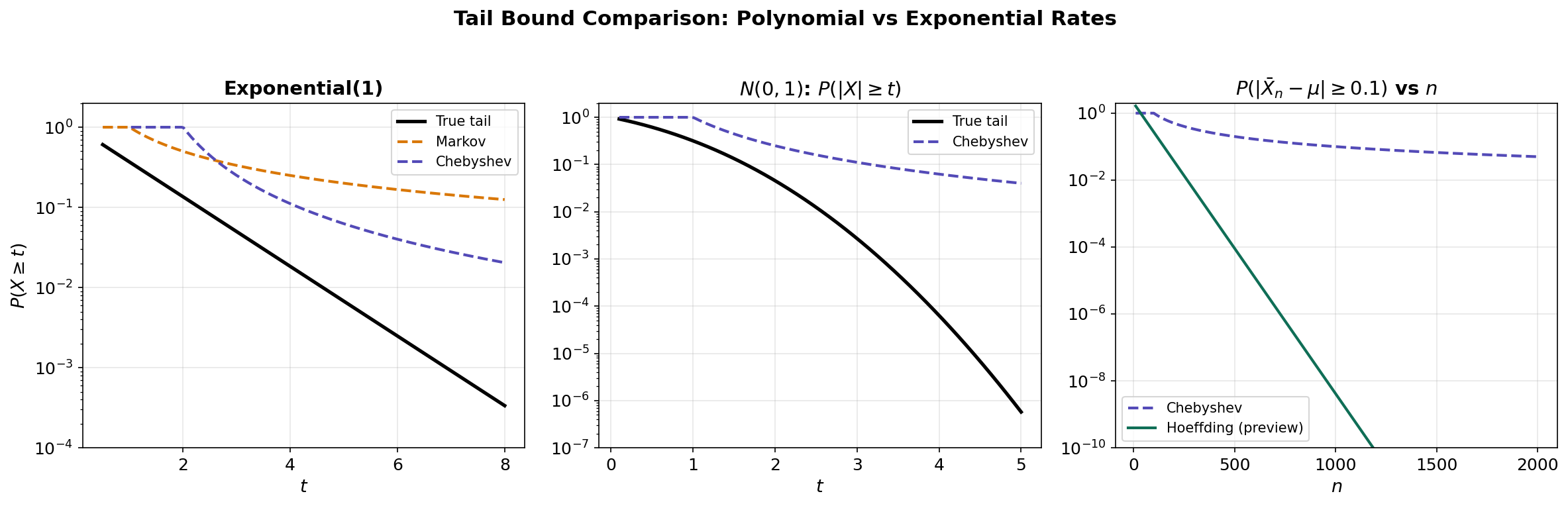
The figure above demonstrates how loose the basic tail bounds are compared to the true tail probability. In the next section, we introduce the key idea that bridges the gap: the Chernoff method.

Tail Bound Explorer

Distribution:Exponential(1)Uniform[0,1]N(0,1)Beta(2,5)δ = 0.05MarkovChebyshevChernoff/Hoeffding

True tail Markov Chebyshev Chernoff

# Tail Bound Comparison: Markov vs Chebyshev vs True Tail
import numpy as np
from scipy import stats
import matplotlib.pyplot as plt

t_vals = np.linspace(0.5, 8, 200)
mu, sigma2 = 1.0, 1.0  # Exp(1): mean=1, var=1

true_tail = np.exp(-t_vals)                           # P(X >= t) = e^{-t}
markov_bound = np.minimum(mu / t_vals, 1.0)           # E[X] / t
chebyshev_bound = np.minimum(sigma2 / (t_vals - mu)**2, 1.0)  # Var / (t - mu)^2

# Chebyshev is only meaningful for t > mu
chebyshev_bound[t_vals <= mu] = 1.0

plt.semilogy(t_vals, true_tail, 'k-', linewidth=2.5, label='True tail')
plt.semilogy(t_vals, markov_bound, '--', color='#D97706', linewidth=2, label='Markov')
plt.semilogy(t_vals[t_vals > mu], chebyshev_bound[t_vals > mu],
             '--', color='#534AB7', linewidth=2, label='Chebyshev')
plt.xlabel('t'); plt.ylabel('P(X >= t)')
plt.title('Exponential(1): Tail Bounds vs True Tail')
plt.legend()

---

The Chernoff Method and Moment Generating Functions

The Key Idea: Exponentiate and Apply Markov

The breakthrough from polynomial to exponential tail bounds comes from a remarkably simple trick: instead of applying Markov directly to $X$, apply it to $e^{\lambda X}$ for an optimized parameter $\lambda > 0$.

The Chernoff Bound

Application to Sums of Independent Variables

For a sum $S_n = X_1 + \cdots + X_n$ of independent random variables, the MGF factorizes:

$M_{S_n}(\lambda) = \prod_{i=1}^n M_{X_i}(\lambda)$

This is because independence gives $E[e^{\lambda S_n}] = E[\prod_i e^{\lambda X_i}] = \prod_i E[e^{\lambda X_i}]$. The log-MGF (cumulant generating function) therefore adds:

$\psi_{S_n}(\lambda) = \sum_{i=1}^n \psi_{X_i}(\lambda)$

This additivity is why the Chernoff method is particularly powerful for sums of independent variables.

The Log-MGF and Cramér’s Theorem (Preview)

The rate function $\psi_X^*(t)$ measures how “surprising” it is to observe $X \geq t$. This connects to large deviations theory and information-theoretic quantities like the KL divergence.

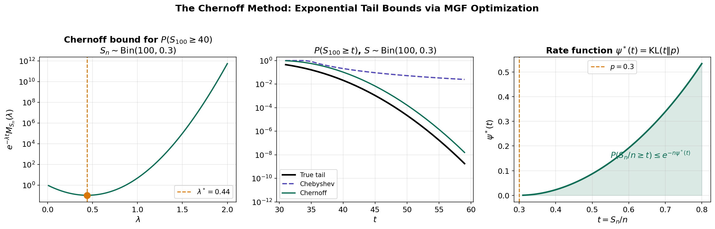
# Chernoff Method: Optimizing the Exponential Tilt
p, n = 0.3, 100
t_target = 40  # P(S_n >= 40) where np = 30

lambdas = np.linspace(0.01, 2.0, 200)
chernoff_bounds = []
for lam in lambdas:
    mgf = (1 - p + p * np.exp(lam))**n
    bound = np.exp(-lam * t_target) * mgf
    chernoff_bounds.append(bound)

chernoff_bounds = np.array(chernoff_bounds)
opt_idx = np.argmin(chernoff_bounds)

# The optimal λ* minimizes the Chernoff bound
print(f"Optimal λ = {lambdas[opt_idx]:.3f}")
print(f"Chernoff bound = {chernoff_bounds[opt_idx]:.2e}")
print(f"True probability = {1 - stats.binom.cdf(39, n, p):.2e}")

---

Hoeffding’s Inequality

The Chernoff method is powerful but requires computing the MGF of each distribution. Hoeffding’s inequality provides a distribution-free exponential bound for bounded random variables, avoiding the need to compute the specific MGF.

Hoeffding’s Lemma

The key technical ingredient is a bound on the MGF of a bounded, zero-mean random variable.

Hoeffding’s Inequality

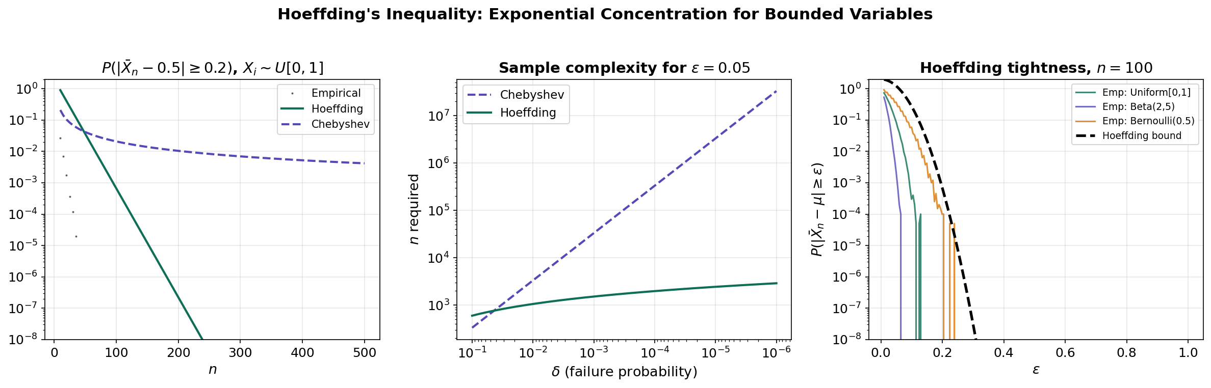
# Hoeffding's Inequality: Empirical Verification
np.random.seed(42)
n_values = np.arange(10, 501, 5)
eps = 0.2
a, b = 0, 1  # Uniform[0,1]
mu, sigma2 = 0.5, 1/12
n_mc = 50000

empirical_probs = []
for n in n_values:
    samples = np.random.uniform(0, 1, (n_mc, n))
    means = samples.mean(axis=1)
    empirical_probs.append(np.mean(np.abs(means - mu) >= eps))

hoeffding_bound = 2 * np.exp(-2 * n_values * eps**2 / (b - a)**2)
chebyshev_bound = np.minimum(sigma2 / (n_values * eps**2), 1.0)

# The Hoeffding bound is a valid upper bound at every n
# Chebyshev is always looser (higher) than Hoeffding

Concentration Rate Demo

Hoeffding Chebyshev

Distribution:Uniform[0,1]Beta(2,5)Bernoulli(0.5)ε = 0.10δ = 0.05Speed:n = 1000

PlayResetNew Sample

---

Sub-Gaussian Random Variables

Hoeffding’s inequality works for bounded random variables, but many important random variables are unbounded (e.g., Gaussian). We need a framework that captures the tail behavior rather than relying on boundedness. This leads to the theory of sub-Gaussian random variables — a class defined by having tails that decay at least as fast as a Gaussian’s.

Motivation

A standard Gaussian $Z \sim N(0, 1)$ has MGF $E[e^{\lambda Z}] = e^{\lambda^2/2}$. The Chernoff method gives:

$P(Z \geq t) \leq e^{-t^2/2}$

This Gaussian tail bound has the form $e^{-ct^2}$. Many distributions — even non-Gaussian ones — exhibit this same qualitative behavior. Sub-Gaussian theory captures this commonality.

Definition and Equivalent Characterizations

Key Examples

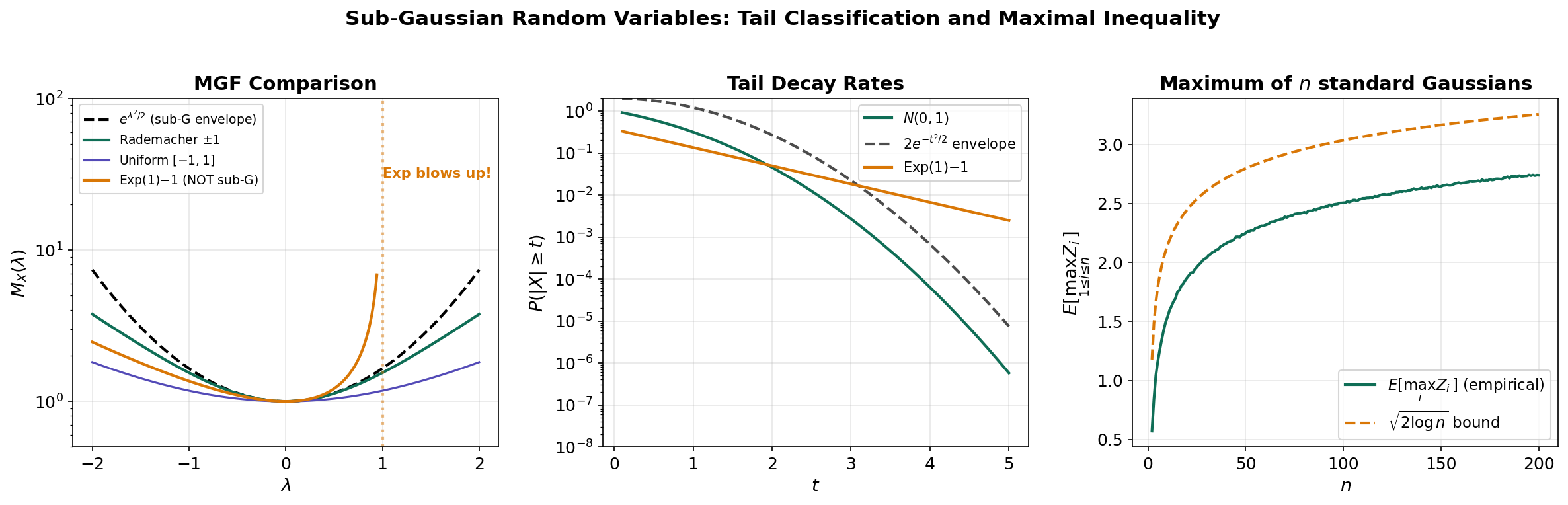
Example 1 (Gaussian). $Z \sim N(0, \sigma^2)$ is $\text{subG}(\sigma^2)$ — the defining example.

Example 2 (Rademacher). $X = \pm 1$ with equal probability. Then $E[e^{\lambda X}] = \cosh(\lambda) \leq e^{\lambda^2/2}$, so $X \sim \text{subG}(1)$.

Example 3 (Bounded). If $a \leq X \leq b$ and $E[X] = 0$, then $X \sim \text{subG}((b-a)^2/4)$ by Hoeffding’s Lemma.

Example 4 (Not sub-Gaussian). $X \sim \text{Exp}(1) - 1$ is not sub-Gaussian: its MGF $E[e^{\lambda X}] = e^{-\lambda}/(1 - \lambda)$ diverges at $\lambda = 1$, so it cannot be bounded by a quadratic for all $\lambda$.

Concentration for Sums of Sub-Gaussians

Maximal Inequality

Sub-Gaussian Classifier

Sub-Gaussian ✓

N(0,1)Rademacher (±1)Uniform[-1,1]Exp(1) − 1t(3)Pareto(2) − 2

---

Sub-Exponential Random Variables and Bernstein’s Inequality

Beyond Sub-Gaussian: Heavier Tails

Not all useful random variables are sub-Gaussian. The centered exponential $X - E[X]$ where $X \sim \text{Exp}(\lambda)$, or the square $Z^2$ of a Gaussian, have tails that decay as $e^{-ct}$ rather than $e^{-ct^2}$. These are sub-exponential random variables.

Bernstein’s Inequality

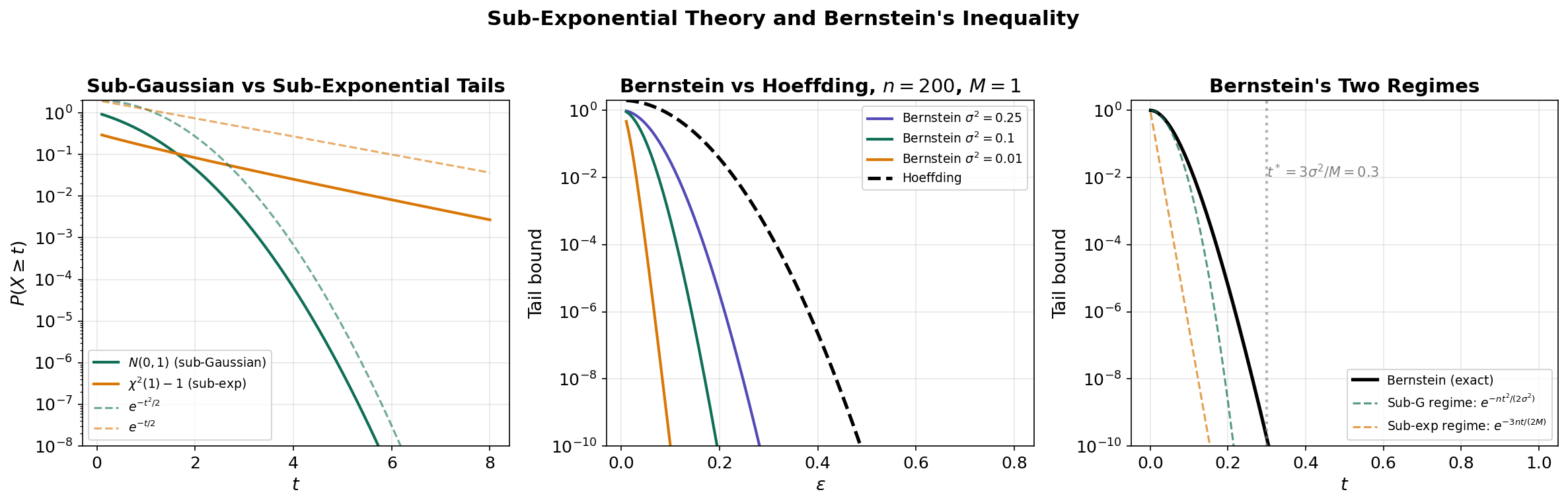
Bernstein’s inequality is sharper than Hoeffding when the variance is small relative to the range. It interpolates between sub-Gaussian behavior (for small deviations) and sub-exponential behavior (for large deviations).

---

McDiarmid’s Inequality

From Sums to General Functions

Hoeffding’s inequality applies to sums $\bar{X}_n = \frac{1}{n}\sum_i X_i$. But in machine learning, we often care about more general functions of independent random variables — for instance, the empirical risk $\hat{R}(h) = \frac{1}{n}\sum_{i=1}^n \ell(h(X_i), Y_i)$, or the supremum of an empirical process $\sup_{h \in \mathcal{H}} |\hat{R}(h) - R(h)|$.

McDiarmid’s inequality extends concentration to any function $f(X_1, \ldots, X_n)$ that doesn’t depend too much on any single coordinate.

The Bounded Differences Condition

McDiarmid’s Inequality

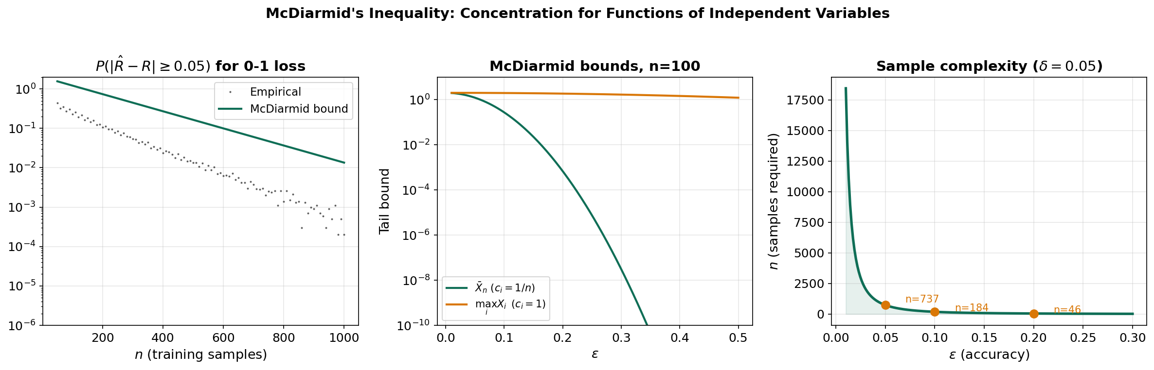
Application: Concentration of Empirical Risk

Example 5 (Empirical Risk). Let $(X_1, Y_1), \ldots, (X_n, Y_n)$ be i.i.d. training samples, $h$ a fixed hypothesis, and $\ell$ a loss function bounded by $M$. Define the empirical risk:

$\hat{R}(h) = \frac{1}{n}\sum_{i=1}^n \ell(h(X_i), Y_i)$

Changing any single sample $(X_i, Y_i)$ changes $\hat{R}(h)$ by at most $M/n$. By McDiarmid:

$P(|\hat{R}(h) - R(h)| \geq \varepsilon) \leq 2\exp(-2n\varepsilon^2/M^2)$

This is the concentration result that enables generalization bounds: the empirical risk concentrates around the true risk at an exponential rate.

---

Applications to Machine Learning

Generalization Bounds for a Fixed Hypothesis

The simplest generalization bound follows directly from Hoeffding’s inequality (or McDiarmid). Given a hypothesis $h$, its true risk $R(h) = E[\ell(h(X), Y)]$ and empirical risk $\hat{R}(h) = \frac{1}{n}\sum_{i=1}^n \ell(h(X_i), Y_i)$, if the loss is bounded by $M$:

The Union Bound and Finite Hypothesis Classes

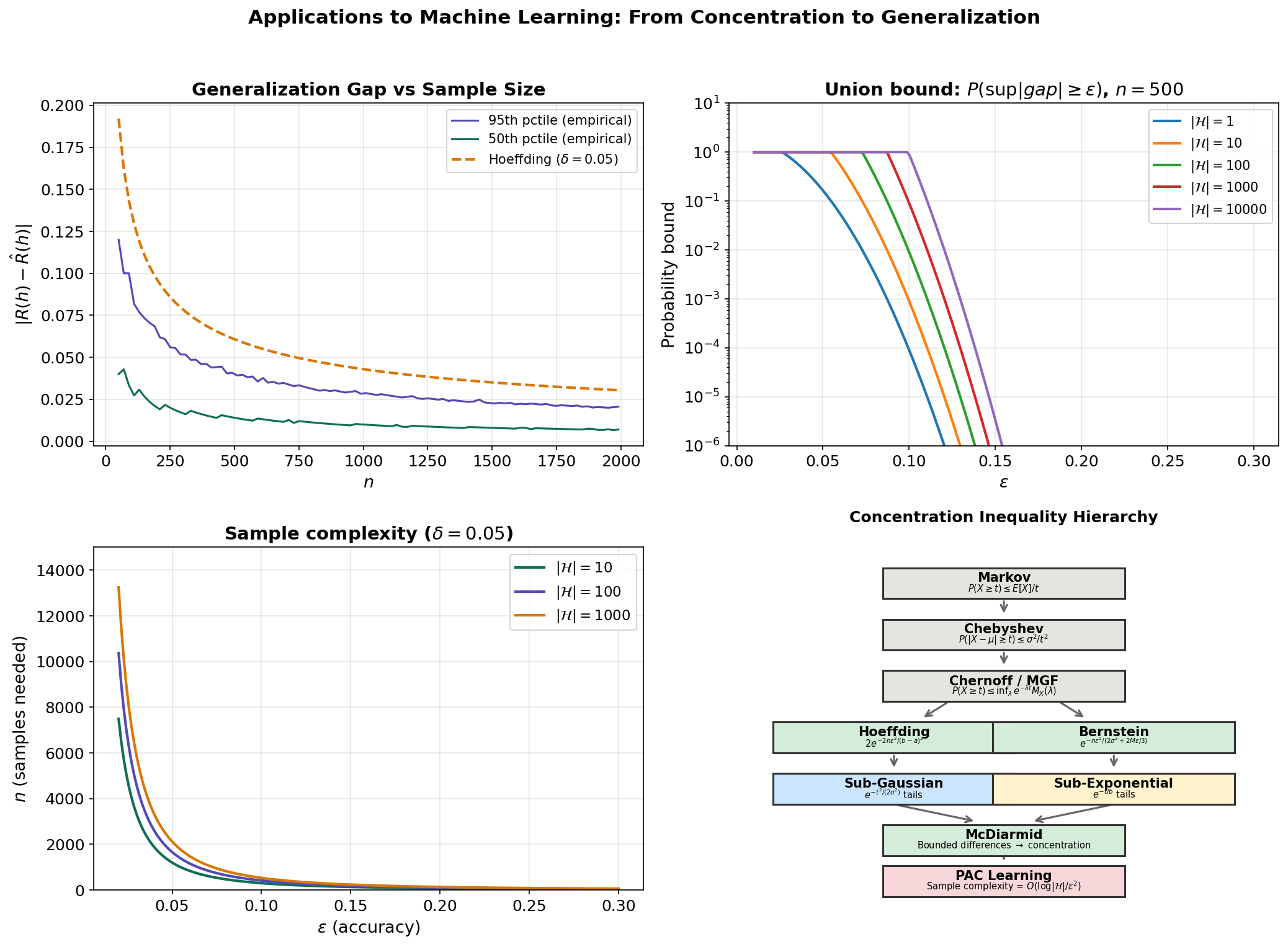
For a finite hypothesis class $\mathcal{H} = \{h_1, \ldots, h_K\}$, we want uniform convergence: $\sup_{h \in \mathcal{H}} |\hat{R}(h) - R(h)| \leq \varepsilon$ simultaneously for all $h$. The union bound (Boole’s inequality) and Hoeffding give:

Sample Complexity

This is the PAC-style sample complexity bound. The dependence on the key parameters is:

• $1/\varepsilon^2$: quadratic in the accuracy — fundamental to most concentration-based bounds.
• $\log|\mathcal{H}|$: logarithmic in the hypothesis class size — the key insight that makes learning tractable.
• $\log(1/\delta)$: logarithmic in the confidence — exponentially better than Chebyshev’s $1/\delta$.

Generalization Bound Calculator

n (samples): 1,000

|H| (hypotheses): 100

δ (failure prob): 0.0501

M (loss bound): 1.0

Generalization bound ε

±0.064

With 1,000 samples and 100 hypotheses, the empirical risk is within ±0.064 of the true risk with 95.0% confidence.

The Bridge to PAC Learning

This section has developed the concentration machinery that the PAC Learning Framework will use extensively. The key ingredients flowing forward are:

1. Hoeffding’s inequality for bounding the gap between empirical and true risk.
2. The union bound for extending single-hypothesis bounds to finite classes.
3. Sub-Gaussian theory as the abstract framework for tail control.
4. McDiarmid’s inequality for concentration of general functions (needed for Rademacher complexity).

The PAC learning framework formalizes this: a hypothesis class $\mathcal{H}$ is PAC-learnable if there exists an algorithm that, given $n \geq n(\varepsilon, \delta, \mathcal{H})$ i.i.d. samples, outputs a hypothesis $\hat{h}$ with $R(\hat{h}) - \inf_{h \in \mathcal{H}} R(h) \leq \varepsilon$ with probability $\geq 1 - \delta$. The sample complexity $n(\varepsilon, \delta, \mathcal{H})$ depends on the “complexity” of $\mathcal{H}$ — measured by VC dimension, Rademacher complexity, or covering numbers — all of which rely on the concentration inequalities developed here.

# Generalization Bounds: Union Bound + Hoeffding for Finite H
np.random.seed(42)
n_vals = np.arange(50, 2001, 20)
true_risk = 0.3
n_mc = 5000

# Empirical generalization gaps (Monte Carlo)
gen_gaps_95 = []
for n in n_vals:
    emp_risks = np.random.binomial(n, true_risk, n_mc) / n
    gaps = np.abs(emp_risks - true_risk)
    gen_gaps_95.append(np.percentile(gaps, 95))

# Hoeffding bound for 95% confidence (delta = 0.05)
hoeffding_95 = np.sqrt(np.log(2 / 0.05) / (2 * n_vals))

# Sample complexity: n >= log(2|H|/delta) / (2 * eps^2)
# For |H| = 100, delta = 0.05:
n_needed = lambda eps: np.log(2 * 100 / 0.05) / (2 * eps**2)

---

Connections & Further Reading

Connections Map

Topic	Domain	Relationship
Measure-Theoretic Probability	Probability & Statistics	Prerequisite — provides $L^p$ spaces, convergence modes, and the expectation operator used throughout
PCA & Low-Rank Approximation	Linear Algebra	Matrix concentration inequalities bound the gap between sample and population covariance eigenvalues
PAC Learning Framework	Probability & Statistics	Direct downstream — uses Hoeffding + union bound for sample complexity; Rademacher complexity uses McDiarmid
Bayesian Nonparametrics (coming soon)	Probability & Statistics	Concentration bounds for posterior contraction rates

Key Notation Summary

Symbol	Meaning
$M_X(\lambda) = E[e^{\lambda X}]$	Moment generating function
$\psi_X(\lambda) = \log M_X(\lambda)$	Cumulant generating function (log-MGF)
$\psi_X^*(t)$	Rate function (Legendre–Fenchel transform)
$\text{subG}(\sigma^2)$	Sub-Gaussian with proxy variance $\sigma^2$
$\|\cdot\|_{\psi_2}$	Sub-Gaussian (Orlicz) norm
$R(h) = E[\ell(h(X), Y)]$	True risk
$\hat{R}(h)$	Empirical risk
$\mathcal{H}$	Hypothesis class