PAC Learning Framework
From finite hypothesis classes to VC dimension and the Fundamental Theorem of Statistical Learning
Overview & Motivation
The Concentration Inequalities topic gave us quantitative tools for controlling how random quantities deviate from their expectations. Hoeffding’s inequality bounds the gap between a sample average and its mean. McDiarmid’s inequality extends this to general functions of independent variables. But those tools answer a specific question — how fast does an average concentrate? — without addressing the deeper question that drives machine learning: when can a learning algorithm generalize at all?
Consider the standard machine learning setup. We have a hypothesis class — a collection of candidate classifiers. We observe a finite training sample and pick the hypothesis that performs best on that sample (empirical risk minimization). The training error is an observable quantity. The true error — performance on unseen data — is not. The gap between them is the generalization gap, and controlling it is the central problem of statistical learning theory.
PAC learning theory answers three fundamental questions:
- Feasibility. For which hypothesis classes is generalization possible — that is, for which can we guarantee that training error approximates true error given enough data?
- Sample complexity. How many training examples suffice to achieve a desired accuracy with confidence ?
- Complexity measures. What properties of determine the answers to (1) and (2)?
We will build the theory in three stages. First, we handle finite hypothesis classes using the concentration tools from the previous topic — the union bound and Hoeffding’s inequality give clean sample complexity bounds. Second, we introduce the VC dimension as the combinatorial measure that governs learnability for infinite classes, and prove the Sauer–Shelah lemma that makes infinite classes tractable. Third, we develop Rademacher complexity as a data-dependent alternative that often gives tighter bounds. The culmination is the Fundamental Theorem of Statistical Learning, which shows these perspectives are equivalent: a hypothesis class is learnable if and only if its VC dimension is finite.
The Learning Problem
We begin by formalizing the setup that machine learning algorithms operate in. The formalization may seem pedantic at first, but each definition isolates an assumption that will matter when we prove our main results.
The setup. We have an instance space (the set of all possible inputs — think feature vectors in ), a label space (binary classification), and an unknown probability distribution over that governs the data-generating process. A hypothesis is a function — a candidate classifier. A hypothesis class is a collection of hypotheses that our learning algorithm considers.
We observe a training sample drawn i.i.d. from . The fundamental tension: we can evaluate how well a hypothesis performs on , but we care about how well it performs on fresh data from .
Definition 1 (True Risk).
The true risk (generalization error) of hypothesis with respect to distribution is:
where is the indicator function that equals 1 when its argument is true and 0 otherwise.
The true risk is the probability of misclassification on a fresh example drawn from . It is the quantity we want to minimize but cannot compute, since is unknown.
Definition 2 (Empirical Risk).
The empirical risk of on sample is:
the fraction of training examples that misclassifies.
The empirical risk is computable — it is the training error. For any fixed hypothesis , the empirical risk is the average of i.i.d. Bernoulli random variables with mean , so by the law of large numbers, as . The question is: does this convergence happen uniformly over all simultaneously, and how fast?
Definition 3 (Empirical Risk Minimization).
The Empirical Risk Minimization (ERM) learning rule selects:
the hypothesis with the lowest training error. When the minimum is achieved by multiple hypotheses, we break ties arbitrarily.
ERM is the most natural learning strategy: pick the hypothesis that fits the training data best. Whether this strategy actually works — whether low training error implies low true error — depends on the hypothesis class , and characterizing when it works is the central goal of PAC theory.
Definition 4 (Realizable Case).
Hypothesis class is realizable with respect to distribution if there exists with . That is, some hypothesis in the class achieves zero true risk — the “ground truth” labeling function belongs to .
Realizability is a strong assumption: it says our hypothesis class is rich enough to contain a perfect classifier. Most real-world problems are not realizable — the best classifier in still makes some errors. We will handle both cases: the realizable setting first (where the analysis is cleaner), then the agnostic setting (where no assumptions are made about ).
Realizable PAC Learning
We are now ready to state the central definition of this topic. The name “PAC” — Probably Approximately Correct — captures both sources of uncertainty: the sample is random (so guarantees are probabilistic, “probably”), and we cannot expect perfect accuracy from finite data (so we settle for approximation, “approximately”).
Definition 5 (PAC Learnability (Realizable)).
A hypothesis class is PAC learnable if there exists a learning algorithm and a function such that for every and every distribution over for which the realizability assumption holds, if , then with probability at least over the random draw of :
The function is the sample complexity of learning .
Let’s unpack this carefully. The definition quantifies over all distributions (where is realizable) and all accuracy/confidence parameters . It asks: is there a single algorithm and a sample size (depending on , and possibly , but not on ) such that produces a hypothesis with true risk at most with high probability? The algorithm does not know — it only sees the sample .
Our first main result shows that every finite hypothesis class is PAC learnable, and ERM is the learning algorithm.
Theorem 1 (PAC Learnability of Finite Classes (Realizable)).
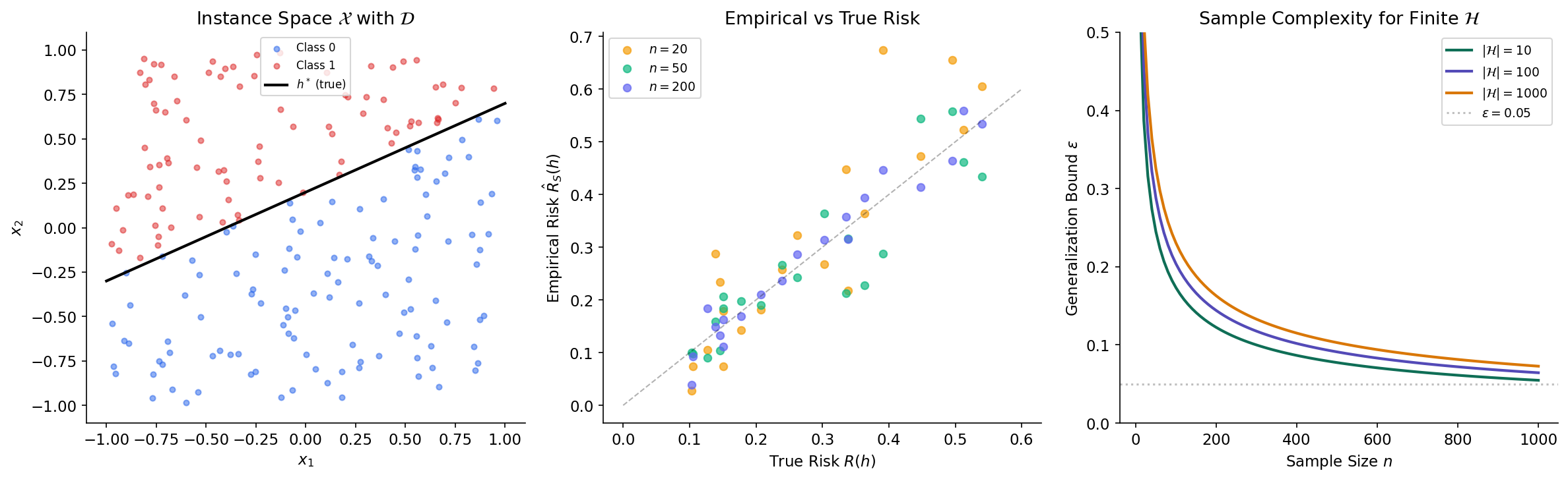
Let be a finite hypothesis class. Then is PAC learnable by ERM with sample complexity:
Proof.
Fix . Let satisfy (this exists by realizability). Define the set of “bad” hypotheses:
Since achieves on any sample (because and the sample is drawn from ), ERM selects some with . The event can only occur if some bad hypothesis has zero empirical risk:
We apply the union bound (from Concentration Inequalities):
For each bad hypothesis with , the event means that correctly classifies all training examples despite having true error greater than . Each training example is correctly classified with probability , and the examples are independent, so:
where the last step uses the standard inequality . Combining:
Setting this to at most and solving for :
∎
Remark (Logarithmic Sample Complexity).
The sample complexity has a clean interpretation. The dependence on is logarithmic — doubling the number of hypotheses adds only one more sample to the requirement. This is the price of the union bound: we pay a log factor to control all hypotheses simultaneously. The dependence on accuracy is — to halve the maximum error, we double the sample size.
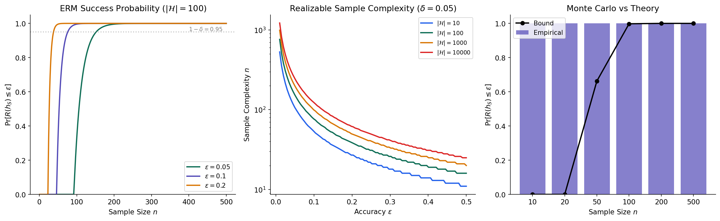
The following code verifies the theoretical bound via Monte Carlo simulation. We create a finite hypothesis class of 50 linear classifiers in , run ERM on random samples of varying sizes, and compare the empirical success probability with the theoretical guarantee.
n_trials = 2000
H_size_sim = 50
d = 5
epsilon_target = 0.1

H_weights = rng.standard_normal((H_size_sim, d))
H_biases = rng.standard_normal(H_size_sim)
h_star_idx = 0  # First hypothesis is the ground truth

sample_sizes_sim = [10, 20, 50, 100, 200, 500]
empirical_success = []

for n_s in sample_sizes_sim:
    successes = 0
    for _ in range(n_trials):
        X_sim = rng.standard_normal((n_s, d))
        y_sim = (X_sim @ H_weights[h_star_idx] + H_biases[h_star_idx] > 0).astype(int)

        # ERM: find hypothesis with lowest training error
        best_h, best_err = None, float('inf')
        for h_idx in range(H_size_sim):
            preds = (X_sim @ H_weights[h_idx] + H_biases[h_idx] > 0).astype(int)
            err = np.mean(preds != y_sim)
            if err < best_err:
                best_err = err
                best_h = h_idx

        # Evaluate true risk on fresh test data
        X_test = rng.standard_normal((5000, d))
        y_test = (X_test @ H_weights[h_star_idx] + H_biases[h_star_idx] > 0).astype(int)
        true_risk = np.mean(
            (X_test @ H_weights[best_h] + H_biases[best_h] > 0).astype(int) != y_test
        )

        if true_risk <= epsilon_target:
            successes += 1

    empirical_success.append(successes / n_trials)

# Compare with theoretical bound: P(success) >= 1 - |H| * exp(-n * epsilon)
theoretical_bound = [
    1 - min(H_size_sim * np.exp(-n_s * epsilon_target), 1.0)
    for n_s in sample_sizes_sim
]
Agnostic PAC Learning
The realizable setting is instructive but unrealistic. In practice, we rarely know whether our hypothesis class contains a perfect classifier. The agnostic setting drops the realizability assumption entirely: the distribution can be arbitrary, and the best hypothesis in may still have nonzero risk. The goal shifts from finding a hypothesis with small absolute risk to finding one whose risk is close to the best achievable within .
Definition 6 (Agnostic PAC Learnability).
A hypothesis class is agnostic PAC learnable if there exists a learning algorithm and a function such that for every and every distribution over (with no realizability assumption), if , then with probability at least :
The term is the approximation error — the best possible risk within — and is the estimation error due to learning from a finite sample.
Remark (Realizable vs Agnostic Rates).
When is realizable, , and agnostic PAC reduces to the realizable definition. But the sample complexity will be different — the agnostic setting requires more samples because we cannot exploit the fact that a perfect hypothesis exists.
The key technique for proving agnostic bounds is uniform convergence: ensuring that empirical risk approximates true risk simultaneously for all hypotheses in .
Proposition 1 (Uniform Convergence Implies Agnostic PAC).
If has the uniform convergence property — that is, for every , there exists such that for :
— then is agnostic PAC learnable by ERM with sample complexity .
Proof.
Suppose uniform convergence holds with parameter , so that for all simultaneously. Let be the ERM hypothesis and . Then:
The first and third inequalities use uniform convergence; the second uses the fact that ERM minimizes empirical risk, so .
∎This proposition reduces the learning problem to a concentration problem: we need to show that uniformly over . For finite classes, this follows directly from Hoeffding’s inequality and the union bound.
Theorem 2 (Agnostic PAC Learnability of Finite Classes).
Let be a finite hypothesis class. Then is agnostic PAC learnable by ERM with sample complexity:
Proof.
We need uniform convergence: with probability at least .
For a fixed hypothesis , the random variables are i.i.d. Bernoulli with mean . By Hoeffding’s inequality (from Concentration Inequalities):
Applying the union bound over all :
Setting this to at most :
By Proposition 1, this gives agnostic PAC learnability with the stated sample complexity.
∎Remark (The 1/ε vs 1/ε² Gap).
Compare the sample complexities: realizable gives while agnostic gives . The agnostic bound is quadratically worse in . This is not an artifact of the proof technique — it reflects a fundamental difference. In the realizable case, we exploited the fact that , which gave us a one-sided tail bound. In the agnostic case, we need a two-sided bound (empirical risk can be both above and below true risk), and controlling this requires the stronger rate from Hoeffding’s inequality.
The following simulation illustrates uniform convergence empirically: we draw 50 random hypotheses, compute their empirical risks over 500 trials, and compare the distribution of the supremum gap against the Hoeffding + union bound prediction.
n_sample = 100
n_hyp = 50
rng2 = np.random.default_rng(123)

true_risks = rng2.beta(2, 5, n_hyp)
emp_risks = np.zeros((n_hyp, 500))

for trial in range(500):
    for h_idx in range(n_hyp):
        outcomes = rng2.binomial(1, true_risks[h_idx], n_sample)
        emp_risks[h_idx, trial] = outcomes.mean()

# Supremum gap over all hypotheses
sup_gap = np.max(np.abs(emp_risks - true_risks[:, None]), axis=0)

# Theoretical bound: Hoeffding + union bound
eps_theory = np.linspace(0.001, 0.4, 200)
p_exceed_hoeffding_ub = np.minimum(
    2 * n_hyp * np.exp(-2 * n_sample * eps_theory**2), 1.0
)

# Empirical exceedance probability for comparison
empirical_survival = [np.mean(sup_gap > e) for e in eps_theory]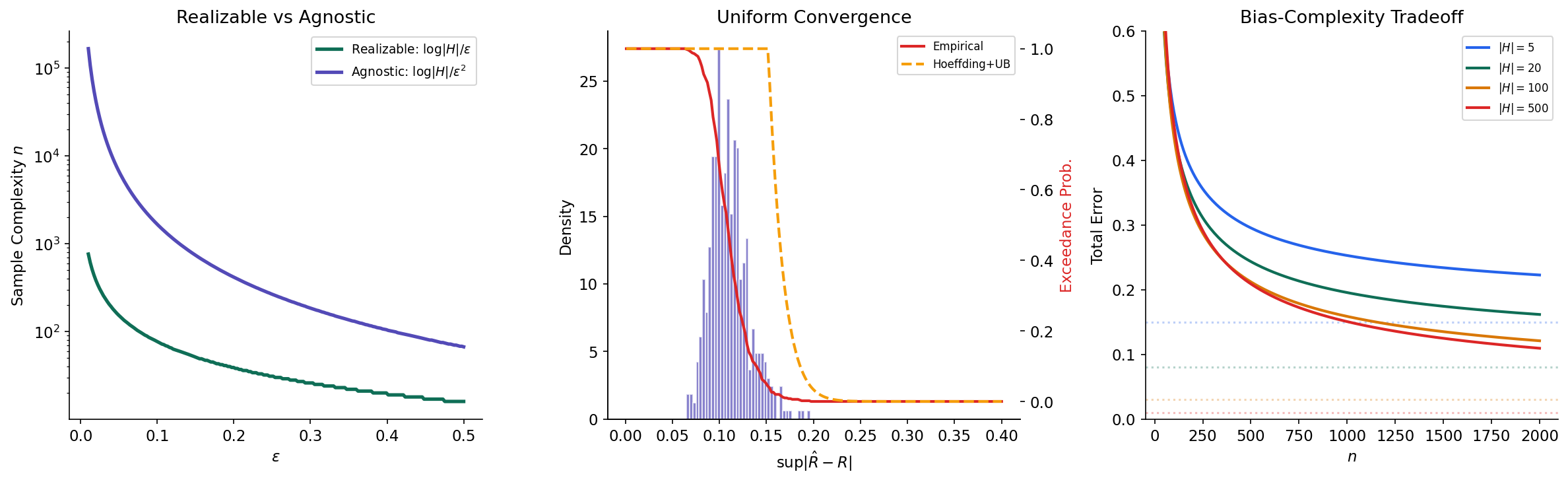
The VC Dimension
For finite hypothesis classes, the story is complete: both realizable and agnostic PAC learning are possible, with sample complexity logarithmic in . But most interesting hypothesis classes are infinite — the class of all linear classifiers in , for instance, has uncountably many elements. The union bound over is useless when .
The key insight is that an infinite hypothesis class, when restricted to a finite sample, can only produce finitely many distinct labeling patterns. The effective complexity of on points is not but the number of distinct behaviors on those points. This leads us to the VC dimension.
Definition 7 (Restriction).
The restriction of hypothesis class to a finite set is:
This is the set of all labeling patterns that hypotheses in can produce on the points in .
Even if is infinite, is always finite — it has at most elements (the total number of possible binary labelings of points). The question is: for how large an can we achieve the maximum ?
Definition 8 (Shattering).
A hypothesis class shatters a set if , i.e., every possible binary labeling of is realized by some .
Shattering means is maximally expressive on — no matter how the points are labeled, some hypothesis in fits perfectly. This is the combinatorial analog of overfitting: if can shatter large sets, it can memorize arbitrary patterns, which makes generalization harder.
Definition 9 (VC Dimension).
The Vapnik–Chervonenkis dimension of , denoted , is the largest integer such that there exists a set with that is shattered by . If can shatter arbitrarily large sets, then .
The VC dimension measures the largest set of points that can label in all possible ways. It is a worst-case combinatorial measure: we only need one set of size that is shattered, but no set of size can be shattered. Let’s see some examples.
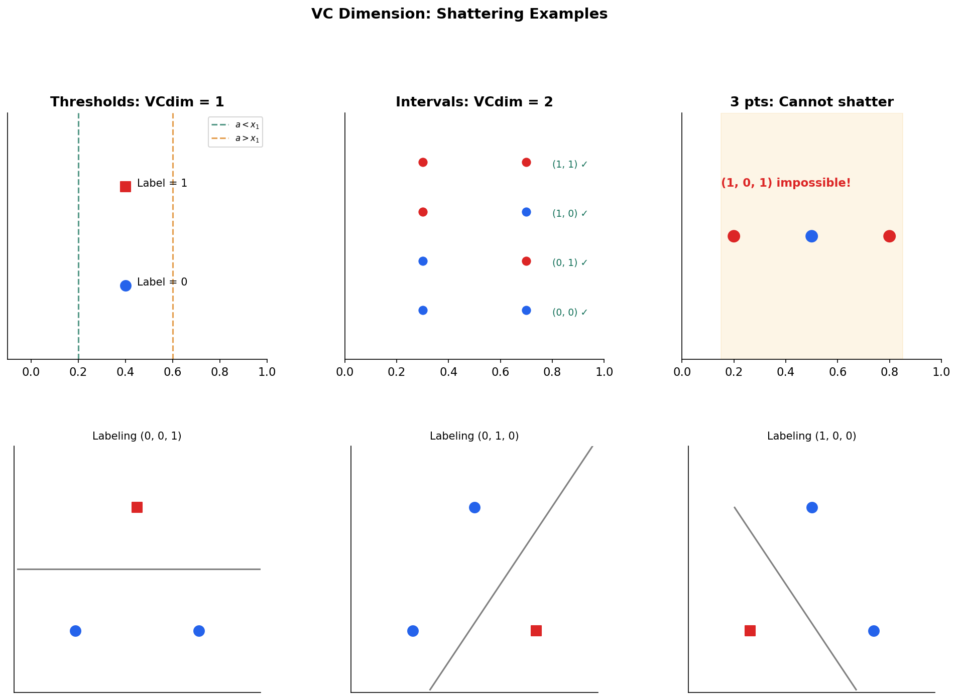
Example 1 (Thresholds on ℝ).
Consider where (predict 1 if is at most ). For any single point , we can realize both labelings: choose for label 1, or for label 0. So shatters sets of size 1.
But for any pair with , the labeling — “the smaller point is negative and the larger point is positive” — cannot be achieved by any threshold. Therefore .
Example 2 (Intervals on ℝ).
Consider where (predict 1 if lies in the interval ). Any two points can be shattered (check all four labelings). But for three points , the labeling — positive at the endpoints, negative in the middle — cannot be produced by a single interval. Therefore .
The most important example for machine learning is linear classifiers, whose VC dimension has a clean characterization.
Theorem 3 (VC Dimension of Linear Classifiers).
The class of halfspaces in :
has .
Proof.
Lower bound (). We exhibit a set of points that shatters. Take the origin and the standard basis vectors . For any binary labeling of these points, we can construct a weight vector and bias that realizes it. The key is that these points are in “general position” — no of them lie on a common hyperplane — so the linear constraints (or ) are always simultaneously satisfiable.
Upper bound (). We use Radon’s theorem from convex geometry: any set of points in can be partitioned into two disjoint sets whose convex hulls intersect: . If the convex hulls intersect, no hyperplane can separate from , so the labeling that assigns 1 to and 0 to is not realizable. Therefore no set of points can be shattered.
∎This result connects the VC dimension to the geometric dimension of the feature space: linear classifiers in have VC dimension . This is why the number of features matters for generalization — it directly controls the complexity of the hypothesis class.
Sauer–Shelah Lemma and Growth Functions
The VC dimension tells us the boundary at which shattering becomes impossible: cannot shatter any set of size or larger. But we need a more quantitative statement: exactly how many labelings can produce on a set of points when ? The growth function captures this.
Definition 10 (Growth Function).
The growth function (also called the shattering coefficient) of is:
the maximum number of distinct labelings that can produce on any set of points. By definition, always, and means but for all .
The Sauer–Shelah lemma is the remarkable fact that once drops below , it doesn’t just decrease slightly — it collapses from exponential to polynomial growth. This is the combinatorial engine that makes infinite hypothesis classes learnable.
Lemma 1 (Sauer–Shelah Lemma).
If , then for all :
Proof.
We prove this by strong induction on .
Base cases. If , then cannot shatter any single point, so for all . If , then trivially.
Inductive step. Assume the lemma holds for all pairs with . Let be any set of points achieving the maximum . Set .
We partition based on the behavior at . For each labeling pattern , either:
- extends to exactly one labeling on (either or is in , but not both), or
- extends to both labelings on (both extensions are in ).
Let be the set of all patterns on , and let be the set of patterns that extend both ways. Then:
because each pattern in contributes one labeling on , and each pattern in contributes two.
Now we bound each term:
-
is the restriction of to points, so . By the inductive hypothesis: .
-
For , we claim . If shattered a set of size , then since every pattern in extends both ways on , the set of size would be shattered by — contradicting . By the inductive hypothesis: .
Combining and using Pascal’s identity :
∎
Corollary 1 (Polynomial Growth Bound).
For :
The second inequality follows from the standard bound , which can be proved using the entropy method or direct algebraic manipulation.
The significance of Corollary 1 cannot be overstated. The growth function transitions from (exponential) for to (polynomial in with degree ) for . This phase transition at is what allows the VC theory to work: we can replace in the union bound by , which is polynomial rather than infinite.
The following code computes the growth function exactly and demonstrates the phase transition:
from scipy.special import comb

m_range = np.arange(1, 31)

# Growth function for several VC dimensions
for d in [1, 2, 3, 5, 10]:
    growth = np.array([
        sum(comb(m, i, exact=True) for i in range(d + 1))
        for m in m_range
    ])

# Sauer-Shelah bound tightness
d = 3
m_range2 = np.arange(d, 51)
exact = np.array([
    sum(comb(m, i, exact=True) for i in range(d + 1))
    for m in m_range2
])
upper = (np.e * m_range2 / d) ** d  # Simplified bound

# Phase transition: ratio Pi(m) / 2^m drops at m = d
d_val = 5
m_range3 = np.arange(1, 25)
growth_exact = np.array([
    sum(comb(m, i, exact=True) for i in range(d_val + 1))
    for m in m_range3
])
ratio = growth_exact / 2.0**m_range3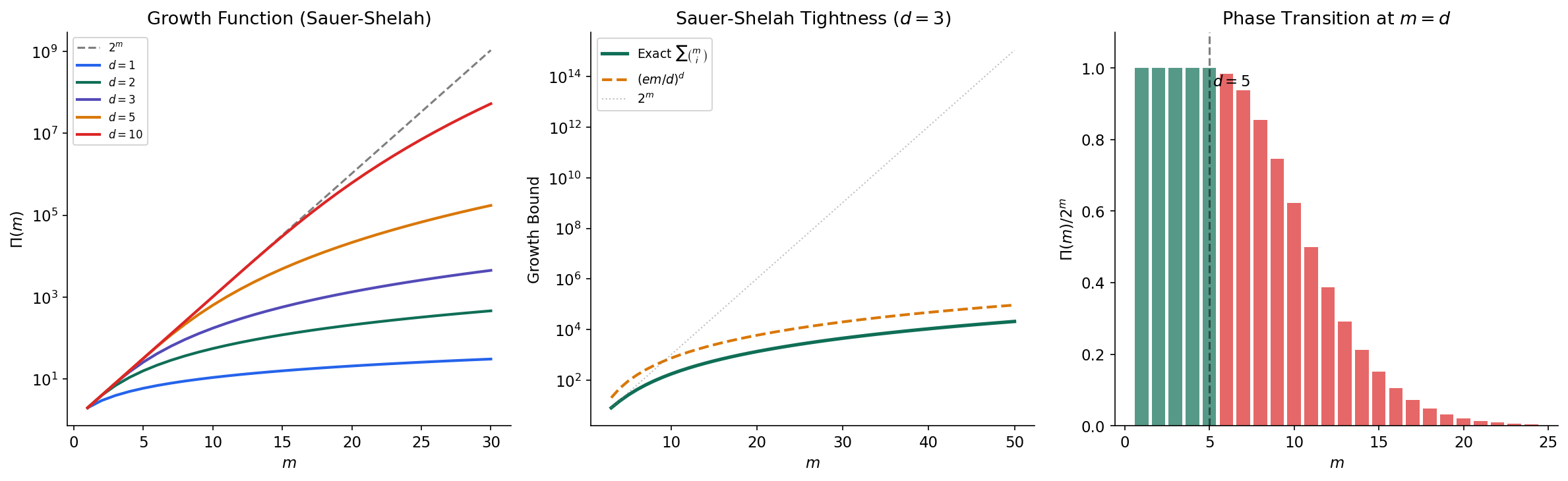
The Fundamental Theorem of Statistical Learning
We now have all the ingredients to state the deepest result in PAC learning theory. The Fundamental Theorem shows that four seemingly different properties of a hypothesis class are equivalent — they are four views of the same underlying phenomenon.
Theorem 4 (VC Bound (Finite-Sample)).
Let . For any distribution and any , with probability at least over :
Proof.
The proof combines three techniques.
Step 1: Symmetrization. Replace the true risk with the empirical risk on an independent “ghost sample” . By a doubling argument, . This step eliminates the unknown distribution from the bound.
Step 2: Rademacher randomization. Since and are exchangeable, we can insert random sign flips: replacing some pairs by doesn’t change the distribution. This yields a bound in terms of Rademacher averages.
Step 3: Growth function bound. On the combined sample of points, produces at most distinct labeling patterns (by Sauer–Shelah). Apply the union bound and Hoeffding’s inequality over these finitely many patterns. The resulting bound is the VC bound.
∎The VC bound establishes uniform convergence for any class with finite VC dimension. Combined with Proposition 1 (uniform convergence implies agnostic PAC), this gives us one direction of the Fundamental Theorem. The full result establishes equivalence.
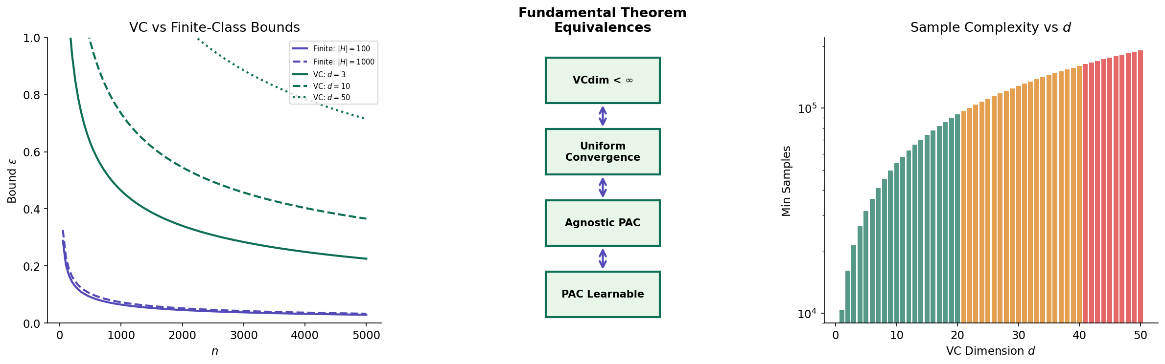
Theorem 5 (The Fundamental Theorem of Statistical Learning).
For binary classification with 0-1 loss, the following are equivalent:
- has the uniform convergence property.
- is agnostic PAC learnable (by ERM).
- is PAC learnable in the realizable setting (by ERM).
- .
Proof.
We outline the implications:
(4) (1): This is Theorem 4 (the VC bound). Finite VC dimension gives us the growth function bound via Sauer–Shelah, which yields uniform convergence through symmetrization and the union bound over distinct labeling patterns.
(1) (2): This is Proposition 1. Uniform convergence guarantees that the ERM hypothesis has risk close to the best in .
(2) (3): Immediate — realizable PAC learnability is a special case of agnostic PAC learnability (set ).
(3) (4): This is the hardest direction, proved by contrapositive. If , then for every sample size , there exists a set of points that shatters. An adversary can construct a distribution on this set such that any learning algorithm fails with probability at least — this is a No Free Lunch argument. The construction places uniform distribution on the points and assigns labels that the adversary chooses after seeing the algorithm’s output, exploiting the shattering to always have a “hard” labeling available.
∎Corollary 2 (VC Dimension Sample Complexity).
If , then is agnostic PAC learnable with sample complexity:
In particular, the sample complexity depends on only through its VC dimension — not on the cardinality or any other structural property of .
Remark (Significance of the Fundamental Theorem).
The Fundamental Theorem is the crown jewel of computational learning theory. It tells us that one number — the VC dimension — completely characterizes whether a binary hypothesis class is learnable. This is a qualitative characterization (finite VC learnable) that also gives quantitative sample complexity bounds (through the VC bound). The elegance is in the equivalence of four seemingly different conditions: a convergence property, two learnability definitions, and a combinatorial measure.
Rademacher Complexity
The VC dimension is a combinatorial complexity measure — it depends on but not on the data distribution or the specific sample . This universality is a strength (the VC bound holds for all distributions) but also a weakness (the bound may be loose for specific distributions). Rademacher complexity provides a data-dependent alternative that can yield tighter bounds.
The intuition is simple: a complex hypothesis class can “fit random noise” — it can correlate with random labels. Rademacher complexity measures this ability.
Definition 11 (Empirical Rademacher Complexity).
For a fixed sample and a function class , the empirical Rademacher complexity is:
where are i.i.d. Rademacher variables: .
The expression inside the expectation asks: given random signs , how well can the best function in correlate with these signs? If contains a function that correlates highly with random noise, the class is complex. If no function can do better than random chance, the class is simple.
Definition 12 (Rademacher Complexity).
The (population) Rademacher complexity is the expectation of the empirical version over the random draw of the sample:
This measures how well can fit random noise on average over samples from .
The main result connects Rademacher complexity to generalization through two applications of concentration inequalities from the previous topic: McDiarmid’s inequality for the concentration step and symmetrization for the expectation bound.
Theorem 6 (Rademacher Generalization Bound).
Let be a class of functions mapping to . For any , with probability at least over :
Proof.
We break the proof into three steps.
Step 1: Bounded differences. Define where . Changing a single sample point changes by at most (since each maps to ). By McDiarmid’s inequality:
Setting gives with probability .
Step 2: Symmetrization. We bound using a ghost sample :
Since and are identically distributed, we can replace by where are Rademacher variables. This gives:
Step 3: Empirical to population. We convert to the empirical using McDiarmid again. The empirical Rademacher complexity has bounded differences (changing one sample point changes the supremum by at most ). So with probability :
Combining Steps 1–3 by a union bound over the two events:
∎
Two structural results connect Rademacher complexity to our earlier measures.
Proposition 2 (Massart's Lemma).
For a finite function class :
where . This recovers the rate for finite classes.
Proposition 3 (VC Bounds Rademacher Complexity).
If , then:
This follows from combining Massart’s Lemma with the Sauer–Shelah bound on the number of effective hypotheses: .
Proposition 3 shows that the Rademacher bound is never worse than the VC bound (up to constants). But because depends on the specific sample , it can be much tighter when the data has favorable structure — for instance, when the data is low-dimensional or when most hypotheses behave similarly on typical inputs.
The following code estimates empirical Rademacher complexity via Monte Carlo simulation:
def estimate_rademacher(H_preds, n_rad=500):
    """
    Estimate empirical Rademacher complexity via Monte Carlo.
    H_preds: (num_hypotheses, sample_size) predictions matrix
    n_rad: number of random sign trials
    Returns: mean of max correlation with random signs
    """
    n_s = H_preds.shape[1]
    maxcorr = []
    for _ in range(n_rad):
        sigma = rng.choice([-1, 1], size=n_s)
        maxcorr.append(np.max(H_preds @ sigma / n_s))
    return np.mean(maxcorr)

# How Rademacher complexity scales with |H|
n_data = 200
X_data = rng.standard_normal((n_data, 2))
H_sizes_test = [5, 10, 25, 50, 100, 200, 500]
rad_c = []

for H_s in H_sizes_test:
    W = rng.standard_normal((H_s, 2))
    b = rng.standard_normal(H_s)
    preds = np.sign(X_data @ W.T + b)
    rad_c.append(estimate_rademacher(preds.T))

# Compare with theoretical: O(sqrt(log|H| / n))
theory_rc = np.sqrt(2 * np.log(np.array(H_sizes_test)) / n_data)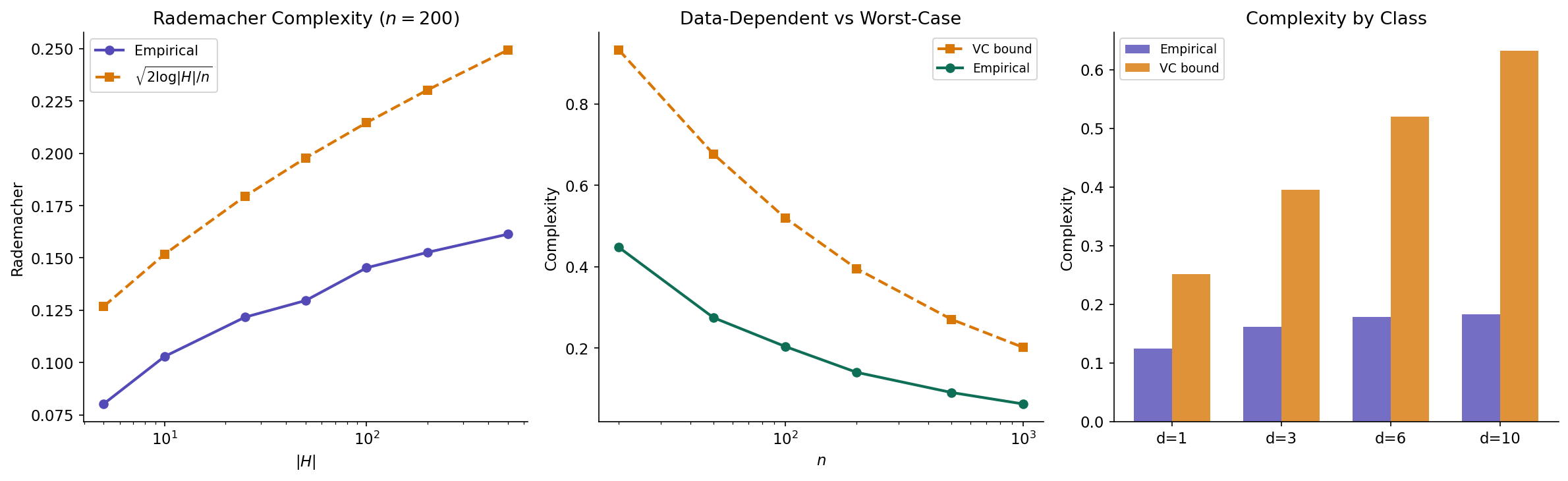
Applications and Worked Examples
The abstract theory developed above has direct implications for understanding the generalization behavior of concrete machine learning methods. We discuss four applications.
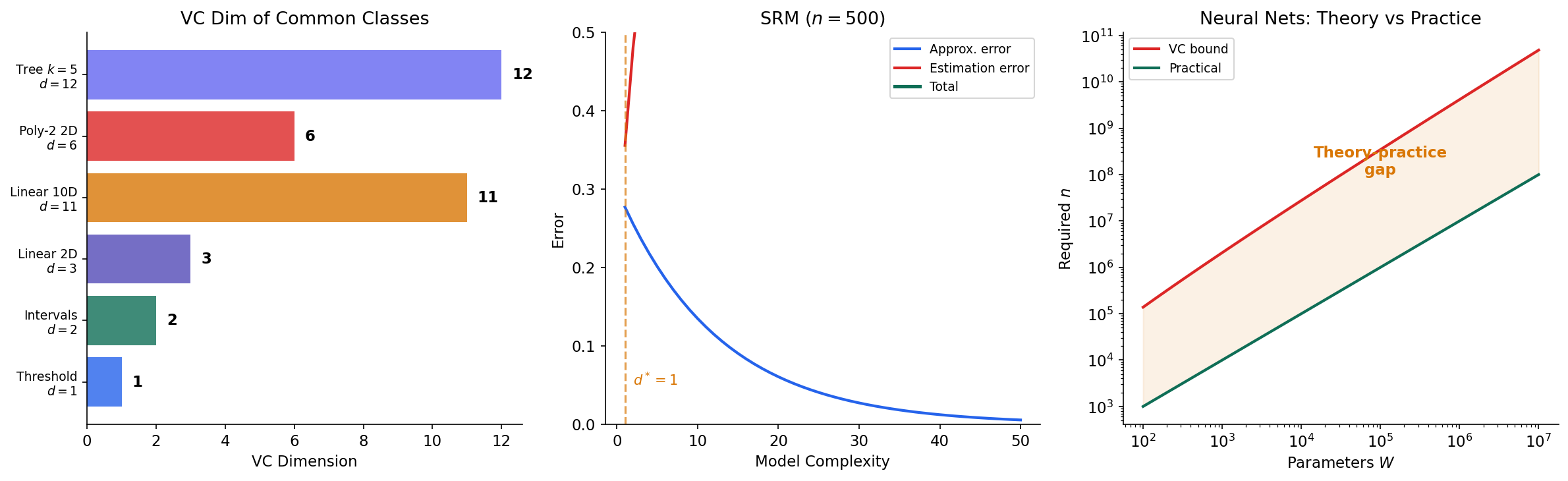
Linear Classifiers
For halfspaces in , we know (Theorem 3). The VC bound gives sample complexity for agnostic PAC learning. This provides a formal justification for the common wisdom that the number of training examples should grow with the number of features. In practice, if we have features and want accuracy, the VC bound suggests we need on the order of samples — conservative, but in the right ballpark for linear methods on moderately difficult problems.
Neural Networks
The VC dimension of a neural network with real-valued weights is (due to Bartlett, Harvey, Liaw & Mehrabian, 2019). For a network with millions of parameters, this gives a sample complexity bound in the millions — but modern networks generalize well with far fewer samples than the VC theory predicts. This theory-practice gap is one of the most active research areas in learning theory. Several explanations have been proposed: the effective capacity of trained networks is much smaller than the architectural capacity, optimization with SGD implicitly regularizes, and the data distribution has favorable structure that tighter measures like Rademacher complexity can exploit.
Decision Trees
A decision tree with internal nodes on -dimensional binary features has VC dimension at most . This shows that the sample complexity scales with the tree complexity (number of splits), not with the ambient dimension . Pruning a decision tree reduces its VC dimension, which the theory predicts should improve generalization — consistent with the well-known observation that unpruned trees overfit.
Structural Risk Minimization
The bias-complexity tradeoff (also called the bias-variance tradeoff in some contexts) is a direct consequence of the PAC framework. Given a nested sequence of hypothesis classes with increasing VC dimensions :
- The approximation error decreases with (larger classes contain better approximations).
- The estimation error (the generalization gap, bounded by the VC bound) increases with (larger classes are harder to learn from finite data).
Structural Risk Minimization (SRM) selects the hypothesis class that minimizes the sum of empirical risk and the VC complexity penalty. This is the learning-theoretic justification for regularization: by controlling model complexity, we balance the two sources of error.
Connections & Further Reading
Connections Map
| Topic | Domain | Relationship |
|---|---|---|
| Concentration Inequalities | Probability & Statistics | Direct prerequisite — Hoeffding + union bound give sample complexity for finite classes; McDiarmid’s inequality proves the Rademacher generalization bound |
| Measure-Theoretic Probability | Probability & Statistics | Foundational — the convergence hierarchy and expectation operator underpin the definitions of true risk and uniform convergence |
| PCA & Low-Rank Approximation | Linear Algebra | The VC dimension of linear subspace classifiers relates to effective dimension captured by PCA; sample covariance concentration connects to agnostic learning bounds |
| Simplicial Complexes | Topology | The combinatorial proof of Sauer–Shelah (induction on point removal) has structural analogues in extremal and topological combinatorics |
| Bayesian Nonparametrics | Probability & Statistics | Bayesian model selection provides an alternative to SRM for balancing model complexity; posterior contraction rates parallel PAC sample complexity |
Key Notation Summary
| Symbol | Meaning |
|---|---|
| True risk (generalization error) | |
| Empirical risk (training error) | |
| Empirical risk minimizer | |
| Sample complexity | |
| Restriction of to set | |
| Vapnik–Chervonenkis dimension | |
| Growth function (shattering coefficient) | |
| Empirical Rademacher complexity | |
| Population Rademacher complexity |
Connections
- Direct prerequisite — Hoeffding's inequality and the union bound give sample complexity for finite classes; McDiarmid's inequality proves Rademacher generalization bounds. concentration-inequalities
- Foundational — the convergence hierarchy and expectation operator underpin the definition of true risk and uniform convergence. measure-theoretic-probability
- The VC dimension of linear subspace classifiers relates to effective dimension captured by PCA; sample covariance concentration connects to agnostic learning bounds. pca-low-rank
- The combinatorial proof of Sauer–Shelah has structural analogues in extremal and topological combinatorics. simplicial-complexes
References & Further Reading
- paper A Theory of the Learnable — Valiant (1984) The foundational PAC learning paper
- book Understanding Machine Learning: From Theory to Algorithms — Shalev-Shwartz & Ben-David (2014) Primary reference — Chapters 2-6 cover all topics in this page
- book Statistical Learning Theory — Vapnik (1998) Comprehensive treatment of VC theory and structural risk minimization
- book Foundations of Machine Learning — Mohri, Rostamizadeh & Talwalkar (2018) Excellent treatment of Rademacher complexity and its applications
- paper Learnability and the Vapnik-Chervonenkis Dimension — Blumer, Ehrenfeucht, Haussler & Warmuth (1989) Early paper connecting VC dimension to PAC learning
- paper On the Density of Families of Sets — Sauer (1972) The original Sauer lemma
- paper Rademacher and Gaussian Complexities: Risk Bounds and Structural Results — Bartlett & Mendelson (2002) Foundational paper on Rademacher complexity bounds