Measure-Theoretic Probability
From sigma-algebras to martingales — the rigorous foundations that underpin modern statistics and machine learning
Overview & Motivation
Why do we need measure theory for probability? The short answer: because naive probability breaks down in continuous settings.
Consider a “uniform” random variable on . We want for subsets . For intervals, this is simple: . But what about arbitrary subsets? Can we assign a “length” (probability) to every subset of while preserving countable additivity?
The answer, due to Vitali (1905), is no — there exist non-measurable sets. This forces us to restrict our attention to a carefully chosen collection of “well-behaved” subsets: a sigma-algebra.
This is not an abstract curiosity. Every time we write , compute a conditional expectation , invoke the law of large numbers, or price a financial derivative, we are relying on measure-theoretic machinery. The Lebesgue integral replaces the Riemann integral because it handles limits of random variables correctly (via the Monotone and Dominated Convergence Theorems). Conditional expectation, defined as a Radon–Nikodym derivative, is the mathematical backbone of filtering, Bayesian inference, and martingale theory. And martingales themselves are the language of fair pricing in mathematical finance.
What We Cover
- Sigma-algebras & Measurable Spaces — the sets we can assign probabilities to, and why we need them.
- Measures & Probability Measures — Kolmogorov’s axioms, Lebesgue measure, and the Cantor set.
- Measurable Functions & Random Variables — formalizing “random quantities” as measurable maps.
- The Lebesgue Integral & Expectation — building the integral from simple functions, with full proofs of MCT and DCT.
- Convergence of Random Variables — the four modes, their hierarchy, the Laws of Large Numbers, and the CLT.
- Product Measures & Fubini’s Theorem — integrating over product spaces and why for independent variables.
- Conditional Expectation & Radon–Nikodym — the deepest idea: conditional expectation as an projection.
- A Preview of Martingales — filtrations, adapted processes, and connections to finance.
Connections
This topic connects to the rest of the formalML curriculum in several directions:
- PCA & Low-Rank Approximation — the sample covariance converges to the population covariance by the Law of Large Numbers; theory guarantees convergence of eigenvalues.
- Concentration Inequalities — builds directly on the spaces and convergence theory developed here, quantifying rates of convergence beyond the LLN.
- PAC Learning Framework (coming soon) — uses measure-theoretic probability to formalize learnability.
- Bayesian Nonparametrics (coming soon) — requires conditional expectation and the Radon–Nikodym theorem for prior specifications on infinite-dimensional spaces.
Sigma-Algebras and Measurable Spaces
Why We Need Sigma-Algebras
The fundamental question of probability is: given a sample space , which subsets can we assign probabilities to?
For finite , the answer is easy: every subset. The power set works. But for uncountable — like or — the power set is too large. Vitali’s 1905 construction shows that no translation-invariant, countably additive measure can be defined on all subsets of . We must restrict to a smaller collection of sets that is still rich enough to do calculus.
The right structure is a sigma-algebra: a collection of subsets closed under complements and countable unions. This is precisely what we need for probability — we want to say “the probability of or ” (unions), “the probability of not ” (complements), and we want these operations to work for countable sequences of events.
Definition 1 (Sigma-algebra).
A sigma-algebra (or -algebra) on a set is a collection satisfying:
- (the whole space is measurable),
- If , then (closure under complements),
- If , then (closure under countable unions).
The pair is a measurable space.
Remark.
Properties (2) and (3) together imply closure under countable intersections (by De Morgan’s laws: ), and property (1) with (2) gives .
Examples on a Finite Set
Let . Three sigma-algebras on :
- Trivial: — we can only say “something happens” or “nothing happens.”
- Partial: — we can distinguish element 1 from the rest.
- Power set: — we can distinguish every element.
The trivial sigma-algebra carries the least information; the power set carries the most. This idea — sigma-algebras as information — is the conceptual key to conditional expectation and filtrations.
Generated Sigma-Algebras and the Borel Sets
Given any collection of subsets of , there is a smallest sigma-algebra containing , written . It is the intersection of all sigma-algebras containing — and since the power set is always a sigma-algebra, this intersection is non-empty.
Definition 2 (Borel sigma-algebra).
The Borel sigma-algebra on , denoted , is the sigma-algebra generated by the open intervals:
Equivalently, . The Borel sigma-algebra contains all open sets, closed sets, countable intersections of open sets ( sets), countable unions of closed sets ( sets), and much more. It is the standard sigma-algebra for probability on .
The Borel sets on are defined analogously: .
Here is a Python implementation that verifies the sigma-algebra axioms on finite sets and computes generated sigma-algebras by closure:
def is_sigma_algebra(omega, F):
    """Verify whether F is a sigma-algebra on omega."""
    omega_set = frozenset(omega)
    F_sets = {frozenset(s) for s in F}

    # Axiom 1: omega in F
    if omega_set not in F_sets:
        return False, "Omega not in F"

    # Axiom 2: closure under complements
    for A in F_sets:
        complement = omega_set - A
        if complement not in F_sets:
            return False, f"Complement of {set(A)} not in F"

    # Axiom 3: closure under (finite, here) unions
    for A in F_sets:
        for B in F_sets:
            if A | B not in F_sets:
                return False, f"Union {set(A)} ∪ {set(B)} not in F"

    return True, "Valid sigma-algebra"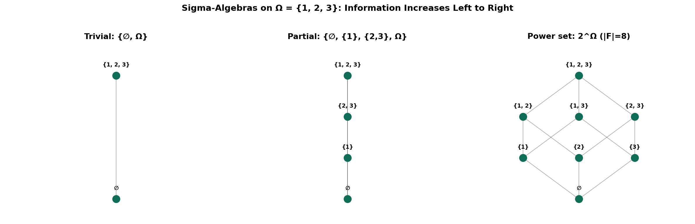
Measures and Probability Measures
Definition of a Measure
A sigma-algebra tells us which subsets are measurable. A measure tells us how big they are.
Definition 3 (Measure).
Let be a measurable space. A measure is a function satisfying:
- (the empty set has zero measure),
- Countable additivity: If are pairwise disjoint, then
The triple is a measure space.
Remark.
Countable additivity is the crucial axiom. Finite additivity ( for disjoint ) is too weak — it cannot guarantee that limits of measurable operations behave well.
Fundamental Properties
Proposition 1 (Monotonicity of measures).
If , then .
Proof.
Write with and disjoint. Then .
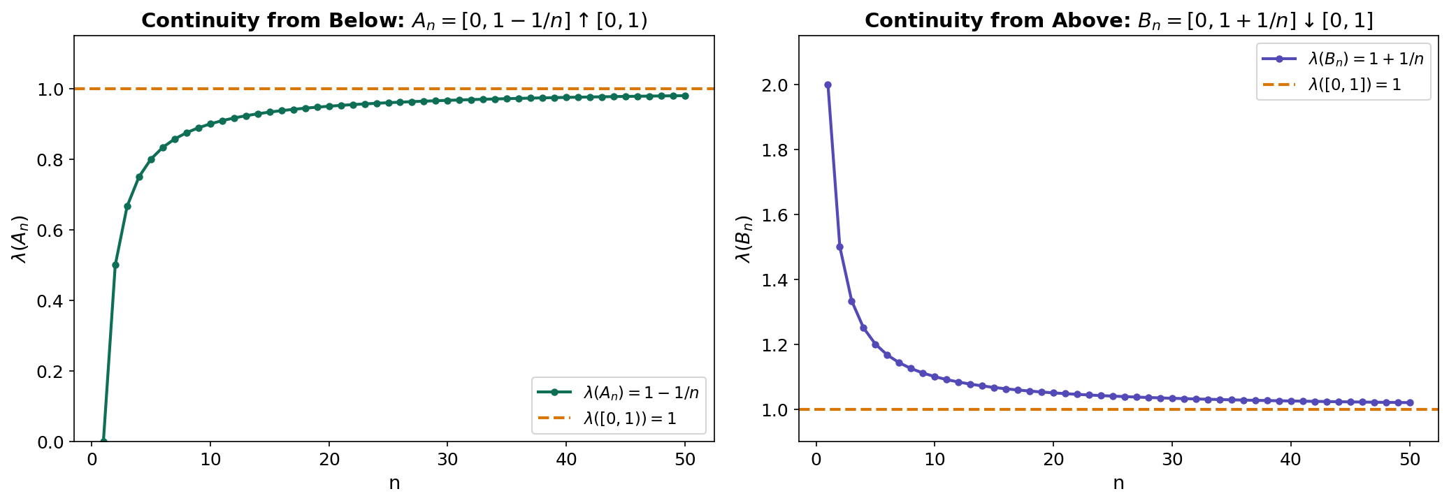
∎Proposition 2 (Continuity from below).
If and , then .
Proof.
Define and for . Then the are pairwise disjoint, , and . By countable additivity:
∎
Proposition 3 (Continuity from above).
If , , and , then .
Proof.
Apply continuity from below to , then use (valid since ).
∎Proposition 4 (Inclusion-exclusion).
For any :
Lebesgue Measure
Definition 4 (Lebesgue measure).
Lebesgue measure on is the unique measure satisfying:
Key properties:
- Translation invariance: for all .
- Scaling: .
- Countable sets have measure zero: .
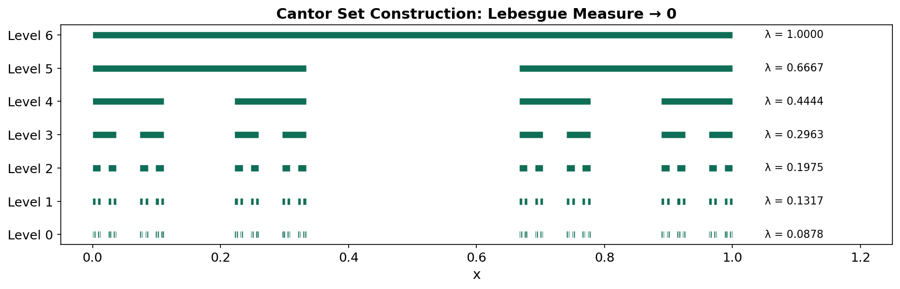
- The Cantor set has measure zero but is uncountable.
The Cantor set is a remarkable object: it is closed, uncountable, has Lebesgue measure zero, and is totally disconnected. We construct it by iteratively removing middle thirds from . At each step, the total length removed is , which converges to — leaving a set of measure zero that still contains uncountably many points (every number in with a ternary expansion using only digits 0 and 2).
Probability Measures and Kolmogorov’s Axioms
Definition 5 (Probability measure).
A probability measure is a measure on with . The triple is a probability space.
Kolmogorov’s axioms (1933) are precisely the axioms for a probability measure:
- for all (non-negativity).
- (normalization).
- for pairwise disjoint (countable additivity).
Every familiar probability distribution defines a probability measure on . The uniform distribution on is simply Lebesgue measure restricted to . A Gaussian defines for Borel sets .
Measurable Functions and Random Variables
Measurable Functions
Definition 6 (Measurable function).
Let and be measurable spaces. A function is -measurable if the preimage of every measurable set is measurable:
Remark.
It suffices to check preimages of a generating collection. For with , it is enough to verify for all .
Proposition 5 (Preservation of measurability).
If and are measurable functions , then so are , , (where ), , , , , and .
Proposition 6 (Limits of measurable functions).
If are measurable, then , , , and are all measurable. In particular, if pointwise, then is measurable.
Proof.
For : we have , which is a countable intersection of measurable sets.
∎Proposition 6 is one of the key advantages of measurable functions over continuous functions: pointwise limits of measurable functions are measurable, while pointwise limits of continuous functions need not be continuous.
Random Variables
Definition 7 (Random variable).
A random variable on a probability space is a measurable function .
This is the measure-theoretic formalization of “a quantity whose value depends on the outcome of a random experiment.” The measurability condition ensures that is well-defined for every Borel set .
A random vector is -measurable. Component-wise: is a random vector if and only if each is a random variable.
Distributions and Independence
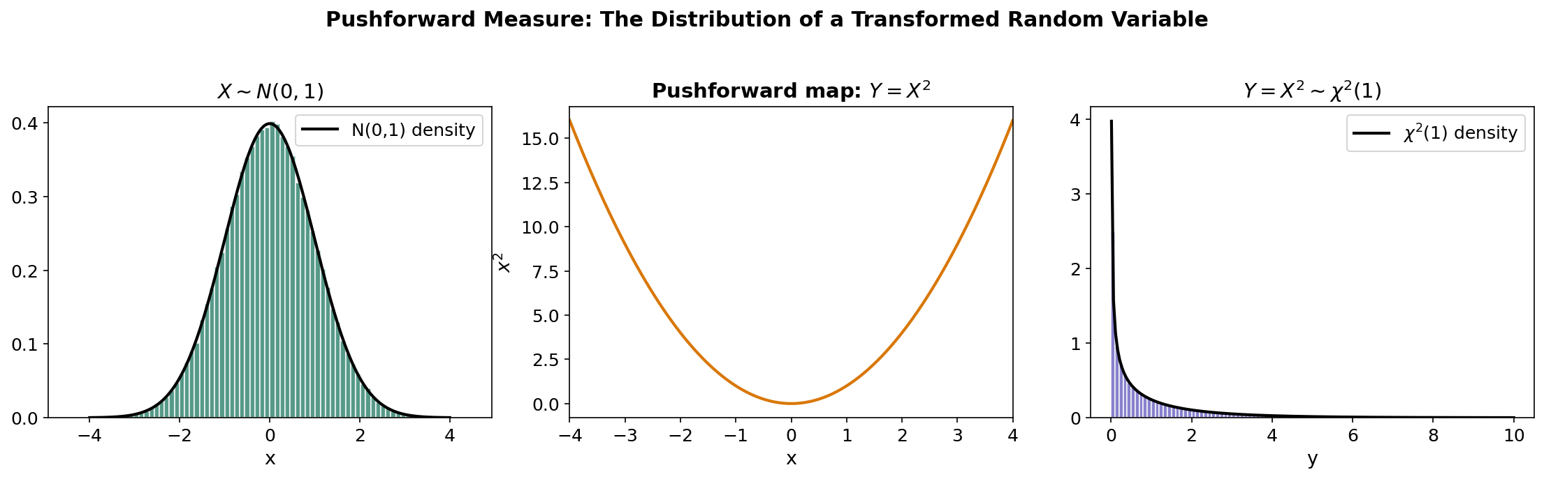
Definition 8 (Law / distribution / pushforward).
The distribution (or law) of a random variable is the probability measure on defined by:
This is the pushforward of by , written or .
The cumulative distribution function (CDF) uniquely determines .
Definition 9 (Independence).
Events are independent if:
Random variables are independent if the sigma-algebras are independent, where .
Equivalently, are independent if and only if the joint CDF factors: .
Remark.
Pairwise vs. mutual independence. Pairwise independence does not imply mutual independence. A classical counterexample: let be independent Rademacher ( with equal probability) and . Then each pair is independent, but has probability .
The Lebesgue Integral and Expectation
Simple Functions and the Construction
The Lebesgue integral is built in three stages: simple functions → non-negative functions → general functions.
Definition 10 (Simple function).
A simple function is a measurable function taking finitely many values. We can write:
where are distinct values and .
Definition 11 (Lebesgue integral of simple functions).
For a non-negative simple function :
Definition 12 (Lebesgue integral (non-negative functions)).
For a measurable :
Definition 13 (Lebesgue integral (general functions)).
For measurable , write where and . Then is integrable (written ) if both and , and:
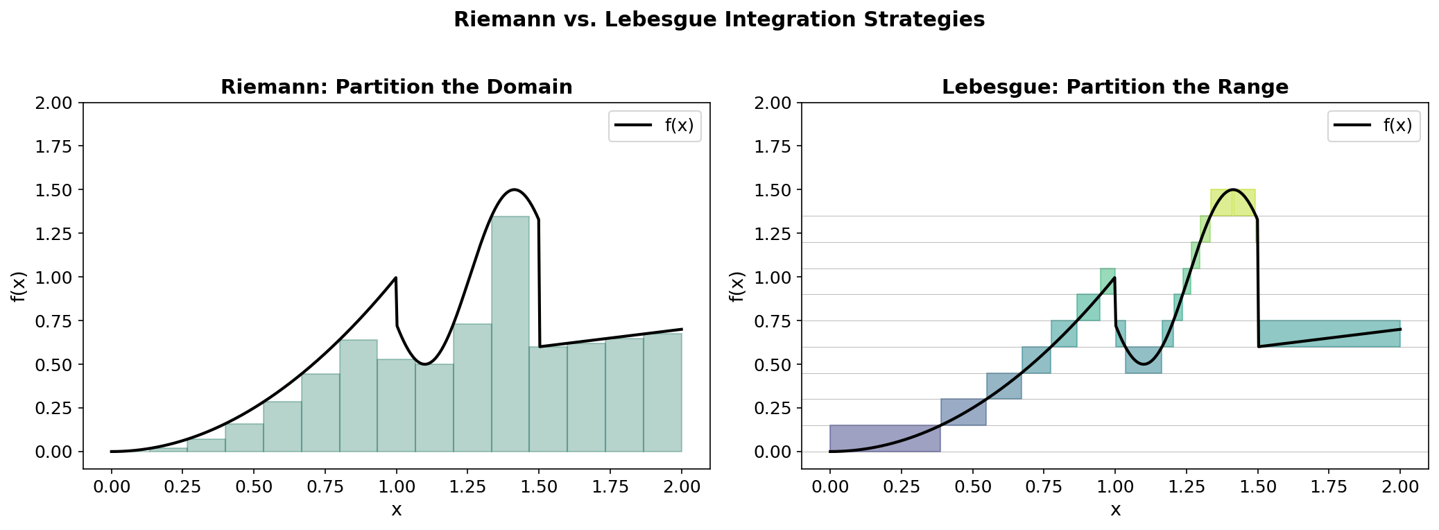
Riemann vs. Lebesgue
The Riemann integral partitions the domain into small intervals and sums . The Lebesgue integral partitions the range into small intervals and sums .
This “horizontal slicing” is why the Lebesgue integral handles limits better: it does not care about the geometric arrangement of the domain, only about the measure of level sets.
The Monotone Convergence Theorem
Theorem 1 (Monotone Convergence Theorem (MCT)).
Let be measurable functions with pointwise. Then:
Proof.
Step 1. Since for all , we have , so .
Step 2. We need to show . Since is the supremum over simple functions , it suffices to show that for any non-negative simple , we have .
Step 3. Fix such a and let . Define . Since on , we have (up to a -null set where ).
Step 4. Then . By continuity from below (applied to the measures ), as :
Since was arbitrary, let to get . Taking the supremum over gives the result.
∎Fatou’s Lemma and the Dominated Convergence Theorem
Lemma 1 (Fatou's Lemma).
If are measurable, then:
Proof.
Define . Then and , so . Apply the MCT to :
∎
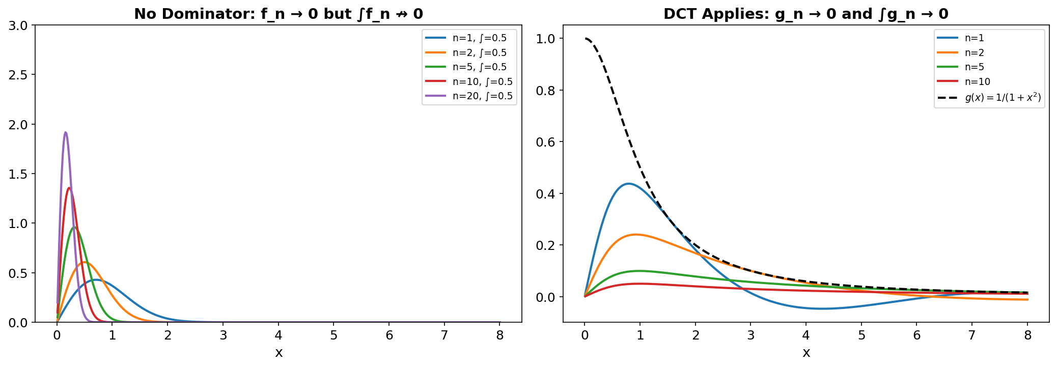
Theorem 2 (Dominated Convergence Theorem (DCT)).
Let pointwise (or -a.e.), and suppose there exists an integrable with for all . Then is integrable and:
Proof.
Since and pointwise, , so . Apply Fatou’s lemma to :
So . Similarly, applying Fatou to :
So . Together: .
∎The DCT is the workhorse of probability theory. Whenever we want to exchange a limit and an integral — which happens constantly in proving convergence results — we look for a dominating function. Without one, the exchange can fail dramatically, as the next example shows.
Expectation and Spaces
Definition 14 (Expectation).
The expectation of a random variable on is:
provided the integral exists. The variance is .
Definition 15 (L^p space).
For , the space consists of all measurable with , with norm:
For : (essential supremum).
Theorem 3 (L^p is a Banach space).
(with functions identified up to -a.e. equality) is a complete normed space.
Theorem 4 (Hölder's inequality).
If with , then:
The case is the Cauchy–Schwarz inequality: . The space is a Hilbert space with inner product .
Convergence of Random Variables
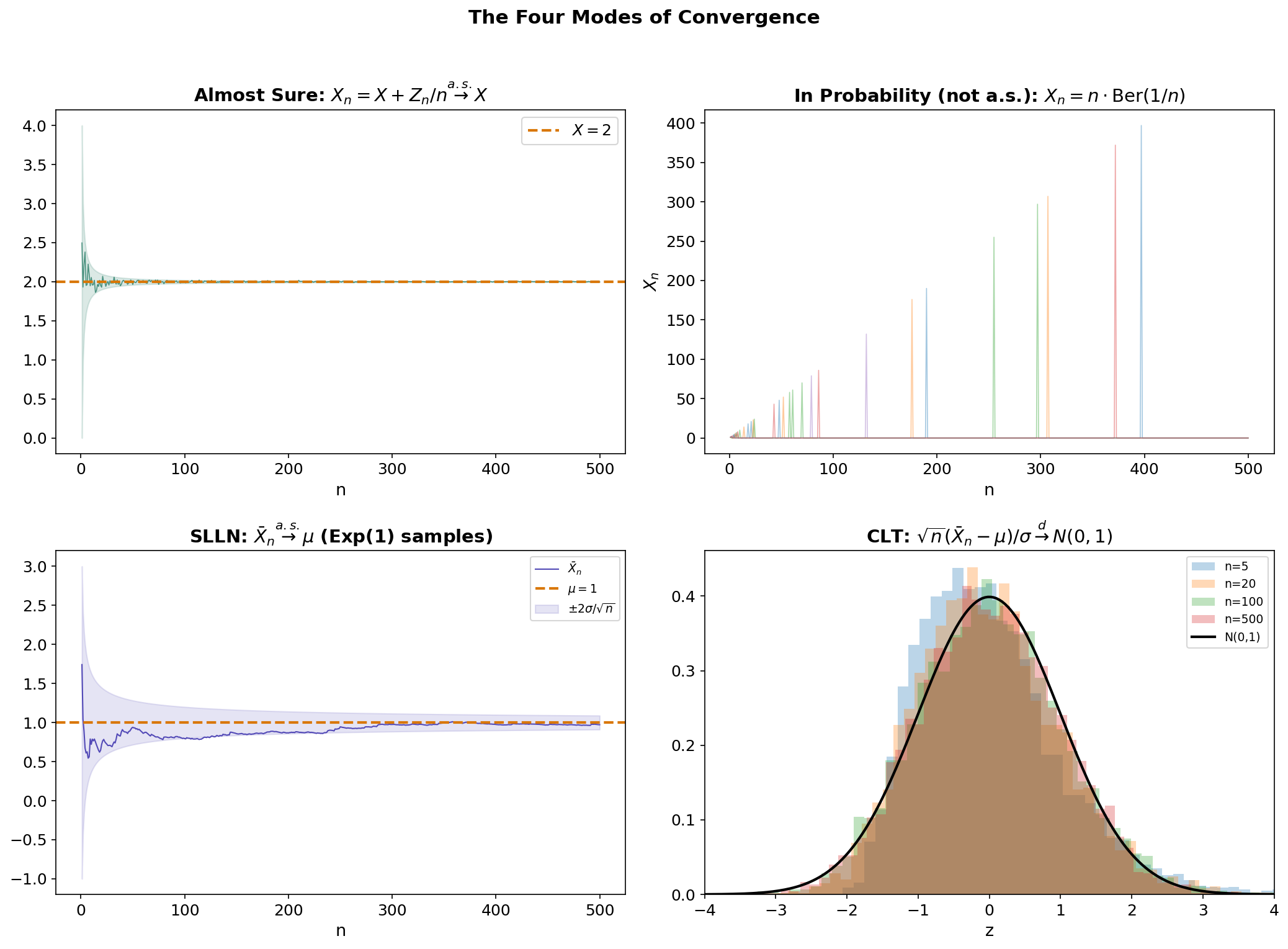
The four modes of convergence — almost sure, in probability, in , and in distribution — form a hierarchy that is central to asymptotic statistics and the theoretical foundations of machine learning.
The Four Modes
Definition 16 (Almost sure convergence).
if:
That is, for almost every outcome , the sequence of numbers converges to .
Definition 17 (Convergence in probability).
if for every :
Definition 18 (Convergence in L^p).
if:
Definition 19 (Convergence in distribution).
if at every continuity point of .
The Hierarchy
The implications between these modes form two chains:
And the converses are generally false, with important exceptions.
Theorem 5 (L^p implies convergence in probability).
Proof.
By Markov’s inequality: .
∎Theorem 6 (Almost sure implies convergence in probability).
Proof.
Define . Almost sure convergence gives (by Borel–Cantelli-type reasoning). Since .
∎Theorem 7 (Convergence in probability implies convergence in distribution).
Proof.
For any continuity point of and :
Letting then gives . A similar lower bound gives the result.
∎Counterexamples
The converses fail in illuminating ways:
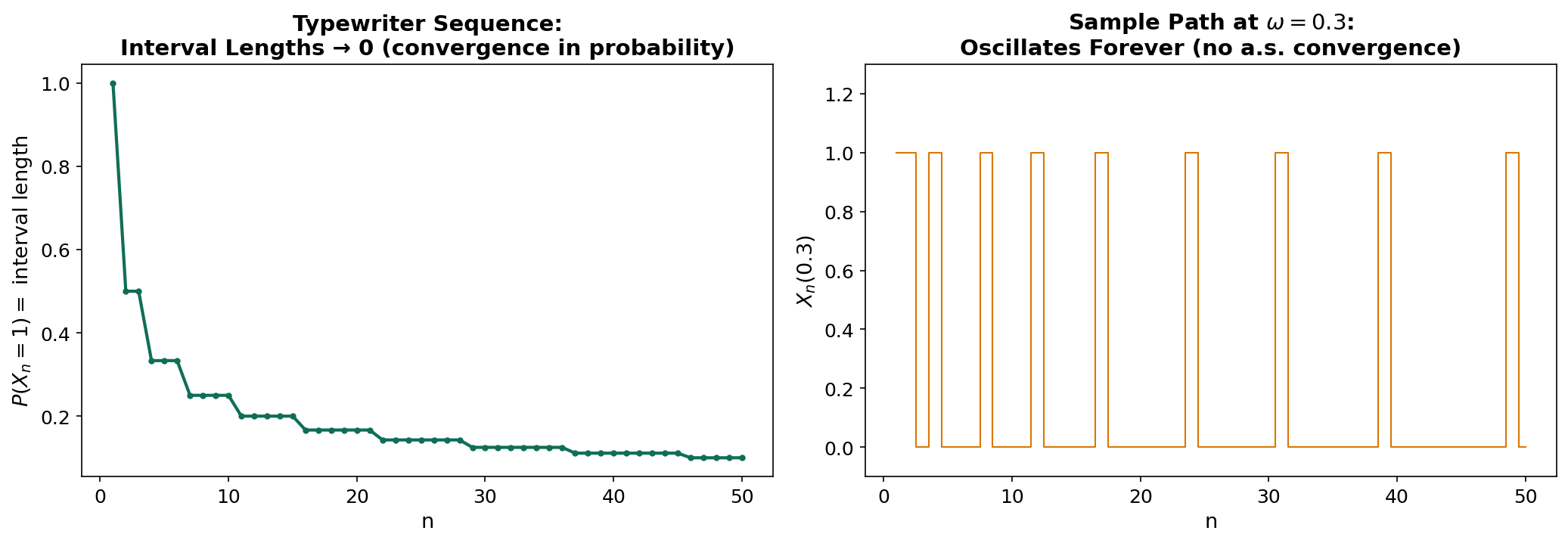
-
In probability does not imply a.s.: The “typewriter sequence” is the classic counterexample. Consider with Lebesgue measure, and define where enumerates pairs by cycling through intervals of decreasing width. Then in probability (the interval width shrinks), but for every , infinitely many .
-
In distribution does not imply in probability: Let and . Then (since too), but for all .
The Laws of Large Numbers
Theorem 8 (Weak Law of Large Numbers (WLLN)).
Let be i.i.d. with and . Then:
Proof.
By Chebyshev’s inequality: .
∎Theorem 9 (Strong Law of Large Numbers (SLLN)).
Let be i.i.d. with and . Then:
The SLLN is strictly stronger than the WLLN: it requires only a finite first moment (not second moment), and the convergence is almost sure. The proof uses the fourth-moment method or truncation arguments and is considerably more involved than the WLLN proof.
The Central Limit Theorem
Theorem 10 (Central Limit Theorem (CLT)).
Let be i.i.d. with and . Then:
The CLT is the deepest result in elementary probability. Its measure-theoretic proof uses characteristic functions: , plus Lévy’s continuity theorem (convergence of characteristic functions if and only if convergence in distribution).
Notice the distinction: the SLLN gives almost sure convergence of to (a constant), while the CLT gives convergence in distribution of the rescaled fluctuations to a Gaussian. These are complementary, not competing, results.
Product Measures and Fubini’s Theorem
Given measurable spaces and , the product sigma-algebra is the sigma-algebra on generated by the measurable rectangles .
Theorem 11 (Product Measure).
If and are -finite measure spaces, there exists a unique measure on satisfying:
For probability spaces, this gives the joint distribution of independent random variables: if and are independent with laws and , then has law .
Theorem 12 (Tonelli's Theorem).
If is -measurable and are -finite, then:
Theorem 13 (Fubini's Theorem).
If additionally is integrable (i.e., ), then the same iterated-integral equalities hold for signed .
Remark.
Tonelli works for non-negative functions without integrability assumptions. Fubini requires integrability but allows signed functions. The standard workflow: use Tonelli to check , then apply Fubini.
Probabilistic consequence. For independent random variables with densities :
and the order of integration can be swapped freely. This is why we can factor joint expectations of independent variables: .
import numpy as np
from scipy import integrate

# Verify Fubini: ∫∫ x²e^{-y} dx dy over [0,1]×[0,∞)
# Iterated integral 1: ∫₀¹ x² dx · ∫₀^∞ e^{-y} dy = (1/3)(1) = 1/3
result_1 = integrate.dblquad(lambda y, x: x**2 * np.exp(-y), 0, 1, 0, np.inf)

# Iterated integral 2 (reversed order)
result_2 = integrate.dblquad(lambda x, y: x**2 * np.exp(-y), 0, np.inf, 0, 1)

print(f"Order 1: {result_1[0]:.6f}")  # 0.333333
print(f"Order 2: {result_2[0]:.6f}")  # 0.333333
Conditional Expectation and Radon–Nikodym
Absolute Continuity and the Radon–Nikodym Theorem
Definition 20 (Absolute continuity).
A measure is absolutely continuous with respect to (written ) if for all .
Theorem 14 (Radon–Nikodym Theorem).
Let and be -finite measures on with . Then there exists a measurable function , unique -a.e., such that:
The function is the Radon–Nikodym derivative .
Proof.
The proof (due to von Neumann) uses the Riesz Representation Theorem on . The functional is bounded on , so by Riesz there exists with . Taking and rearranging yields .
∎If has density with respect to Lebesgue measure , then with . The probability density function is a Radon–Nikodym derivative.
Application to finance. The Radon–Nikodym theorem enables change of measure — the foundation of risk-neutral pricing. If is the real-world measure and is the risk-neutral measure:
This is the mathematical core of the Fundamental Theorem of Asset Pricing.
Conditional Expectation
The measure-theoretic definition of conditional expectation is one of the deepest ideas in probability. We cannot define as a single number — it is a random variable that is -measurable, capturing the “best prediction of given the information in .”
Definition 21 (Conditional expectation).
Let and let be a sub-sigma-algebra. The conditional expectation is the (a.s. unique) -measurable random variable satisfying:
Existence. This follows from the Radon–Nikodym theorem. Define on . Then , and .
Properties of Conditional Expectation
Proposition 7 (Properties of conditional expectation).
Let and be sub-sigma-algebras with .
- Linearity: .
- Tower property: .
- Taking out what is known: If is -measurable and , then .
- Independence: If is independent of , then .
- Trivial conditioning: .
- Full conditioning: .
- Jensen’s inequality: If is convex, then .
Proof (Tower property).
We must show that satisfies the defining property for . For any :
Since , we have , so by the definition of :
And by the definition of : .
So for all , which means satisfies the defining property for . By a.s. uniqueness, they are equal.
∎Conditional Expectation as Projection
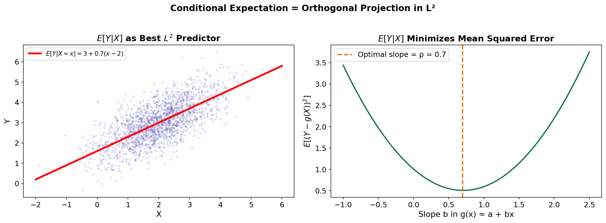
Here is the connection that ties conditional expectation to the Linear Algebra track. The conditional expectation is the orthogonal projection of onto — the subspace of -measurable square-integrable random variables.
Theorem 15 (L^2 projection characterization).
If , then is the unique element minimizing:
Proof.
We verify the orthogonality condition. For any :
By the “taking out what is known” property: (using the tower property at the last step). So — the residual is orthogonal to every -measurable function.
∎This connects directly to PCA: PCA projects data onto a low-dimensional subspace that minimizes mean squared error. Conditional expectation is the infinite-dimensional analog — projecting onto the subspace of functions measurable with respect to a sub-sigma-algebra.
For jointly normal with correlation , the conditional expectation takes the familiar regression form: . The variance reduction is — exactly the fraction of variance “explained” by the conditioning.
import numpy as np

# Conditional expectation as L² projection for jointly normal (X, Y)
np.random.seed(42)
n = 5000
rho = 0.7
mu_x, mu_y, sigma_x, sigma_y = 2.0, 3.0, 1.0, 1.0

# Generate bivariate normal
Z1, Z2 = np.random.randn(n), np.random.randn(n)
X = mu_x + sigma_x * Z1
Y = mu_y + sigma_y * (rho * Z1 + np.sqrt(1 - rho**2) * Z2)

# E[Y | X = x] = mu_y + rho * (sigma_y / sigma_x) * (x - mu_x)
slope = rho * sigma_y / sigma_x
Y_hat = mu_y + slope * (X - mu_x)

# Verify: MSE is minimized at the conditional expectation
mse_optimal = np.mean((Y - Y_hat)**2)
mse_mean_only = np.mean((Y - mu_y)**2)
variance_reduction = 1 - mse_optimal / mse_mean_only

print(f"MSE (conditional): {mse_optimal:.4f}")    # ≈ σ_y²(1-ρ²) = 0.51
print(f"MSE (unconditional): {mse_mean_only:.4f}")  # ≈ σ_y² = 1.0
print(f"Variance reduction: {variance_reduction:.4f}")  # ≈ ρ² = 0.49
A Preview of Martingales
Filtrations and Adapted Processes
Definition 22 (Filtration).
A filtration on is an increasing sequence of sub-sigma-algebras:
Each represents the information available at time . The filtration models the flow of information over time.
Definition 23 (Adapted process).
A sequence of random variables is adapted to a filtration if is -measurable for each . In words: at time , we can observe (it depends only on information available at time ).
The natural filtration of is — the sigma-algebra generated by the first observations. This is the minimal filtration to which is adapted.
Martingales
Definition 24 (Martingale).
An adapted, integrable process is a martingale with respect to if:
If replaces , we have a supermartingale (expected to decrease). If , a submartingale (expected to increase).
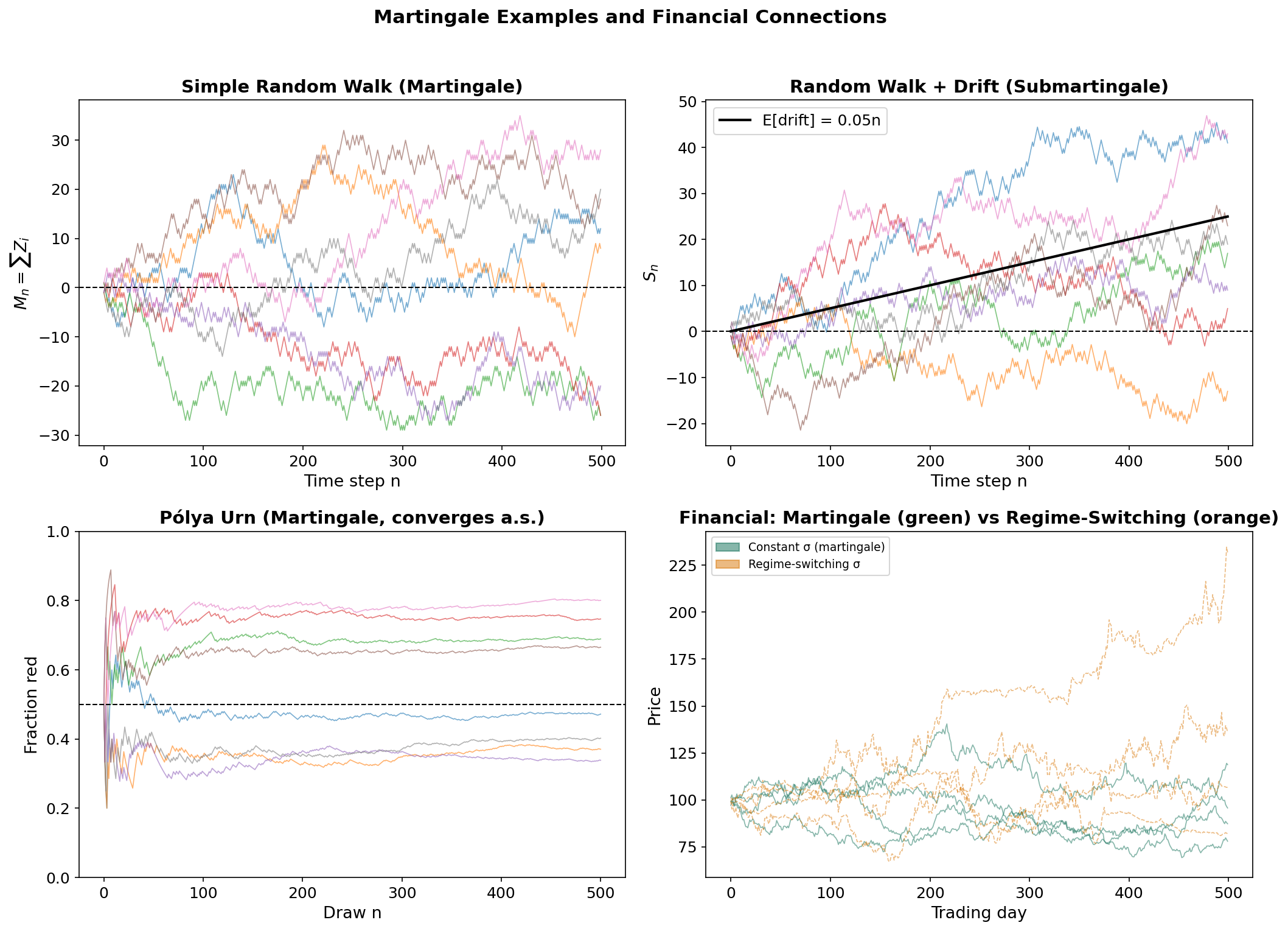
The martingale condition says: given everything we know now, our best prediction of tomorrow’s value is today’s value. The process has “no drift” — no systematic tendency to increase or decrease.
Examples
Random walk. Let be i.i.d. with . Then is a martingale:
using the “taking out what is known” property and independence.
Pólya urn. Start with 1 red and 1 blue ball. At each step, draw a ball, then replace it with 2 balls of the same color. Let = fraction of red balls after draws. Then is a martingale — and by the martingale convergence theorem, converges almost surely to a random variable.
Likelihood ratio. If and are probability measures with , and are i.i.d. under , then the likelihood ratio is a -martingale. This connects to sequential hypothesis testing and the Radon–Nikodym derivative from the previous section.
Financial Interpretation
In mathematical finance, a martingale models a fair game — a process where no betting strategy can generate a positive expected profit.
- A discounted asset price is a martingale under the risk-neutral measure (Fundamental Theorem of Asset Pricing).
- The Efficient Market Hypothesis (weak form) asserts that prices, conditioned on historical information, should be martingales.
- In regime detection, the question is whether the martingale property holds uniformly or whether the drift switches between regimes. GARCH(1,1) captures time-varying conditional variance ( is -measurable), while the Statistical Jump Model detects changes in the conditional distribution itself.
Connections & Further Reading
Cross-Track and Within-Track Connections
| Target | Track | Relationship |
|---|---|---|
| PCA & Low-Rank Approximation | Linear Algebra | converges to by LLN; theory guarantees convergence of eigenvalues |
| Concentration Inequalities | Probability & Statistics | Builds on spaces and convergence theory to quantify rates of convergence beyond LLN |
| PAC Learning Framework | Probability & Statistics | Uses measure-theoretic probability to formalize learnability |
| Bayesian Nonparametrics | Probability & Statistics | Requires conditional expectation, Radon–Nikodym, and product measures for priors on infinite-dimensional spaces |
| Shannon Entropy & Mutual Information | Information Theory | Entropy is , directly using the expectation and Radon–Nikodym machinery developed here. Differential entropy requires the Lebesgue integral; conditional entropy uses conditional expectation. |
| Categories & Functors | Category Theory | The category Meas of measurable spaces and measurable functions provides the categorical framework for probability theory. Random variables are morphisms in Meas, and the pushforward of probability measures is functorial. |
Financial Applications
| Application | Connection |
|---|---|
| GARCH(1,1) | Conditional variance is filtration-adapted |
| Statistical Jump Model | Regime probabilities are conditional expectations given observed filtration |
| Option pricing (Black–Scholes) | Discounted prices are -martingales; is state price density |
| Efficient Market Hypothesis | Prices form martingale w.r.t. public information filtration |
Notation Reference
| Symbol | Meaning |
|---|---|
| Probability space | |
| Borel sigma-algebra on | |
| Lebesgue measure | |
| Indicator function of set | |
| Positive part | |
| Space of -integrable functions | |
| Conditional expectation | |
| Radon–Nikodym derivative | |
| , , , | Modes of convergence |
Connections
- The sample covariance matrix converges to the population covariance by the Law of Large Numbers; L2 theory guarantees convergence of eigenvalues. pca-low-rank
References & Further Reading
- book Probability: Theory and Examples — Durrett (2019) Primary reference — standard graduate probability textbook
- book Probability and Measure — Billingsley (2012) Careful measure-theoretic development
- book Probability with Martingales — Williams (1991) Excellent introduction to martingale theory
- book Real Analysis — Folland (2013) Standard reference for Lebesgue integration and Lp spaces
- book Measure Theory and Probability Theory — Athreya & Lahiri (2006) Balanced between measure theory and probability
- book A Probability Path — Resnick (2014) Transition from undergraduate to measure-theoretic probability
- book Stochastic Calculus for Finance — Shreve (2004) Martingale theory applied to financial mathematics