Graph Laplacians & Spectrum
The eigenvalues and eigenvectors of graph Laplacians — from connectivity to clustering to graph neural networks
Overview & Motivation
A graph encodes pairwise relationships: who knows whom, which proteins interact, which cities are connected by flights. The adjacency matrix records these relationships, but it is the Laplacian that reveals the graph’s deeper structure.
Why the Laplacian and not the adjacency matrix? Because the Laplacian is a real symmetric positive semidefinite matrix, and the Spectral Theorem guarantees it has a complete orthonormal eigenbasis with non-negative eigenvalues. These eigenvalues encode global properties that are invisible to local inspection:
- How many pieces? The multiplicity of the zero eigenvalue equals the number of connected components.
- How well-connected? The second-smallest eigenvalue — the Fiedler value or algebraic connectivity — quantifies the graph’s bottleneck.
- Where to cut? The eigenvector corresponding to — the Fiedler vector — identifies the optimal bipartition.
- How regular? The entropy of the random walk’s stationary distribution, connected to the spectrum via Shannon Entropy, measures how uniformly the graph distributes flow.
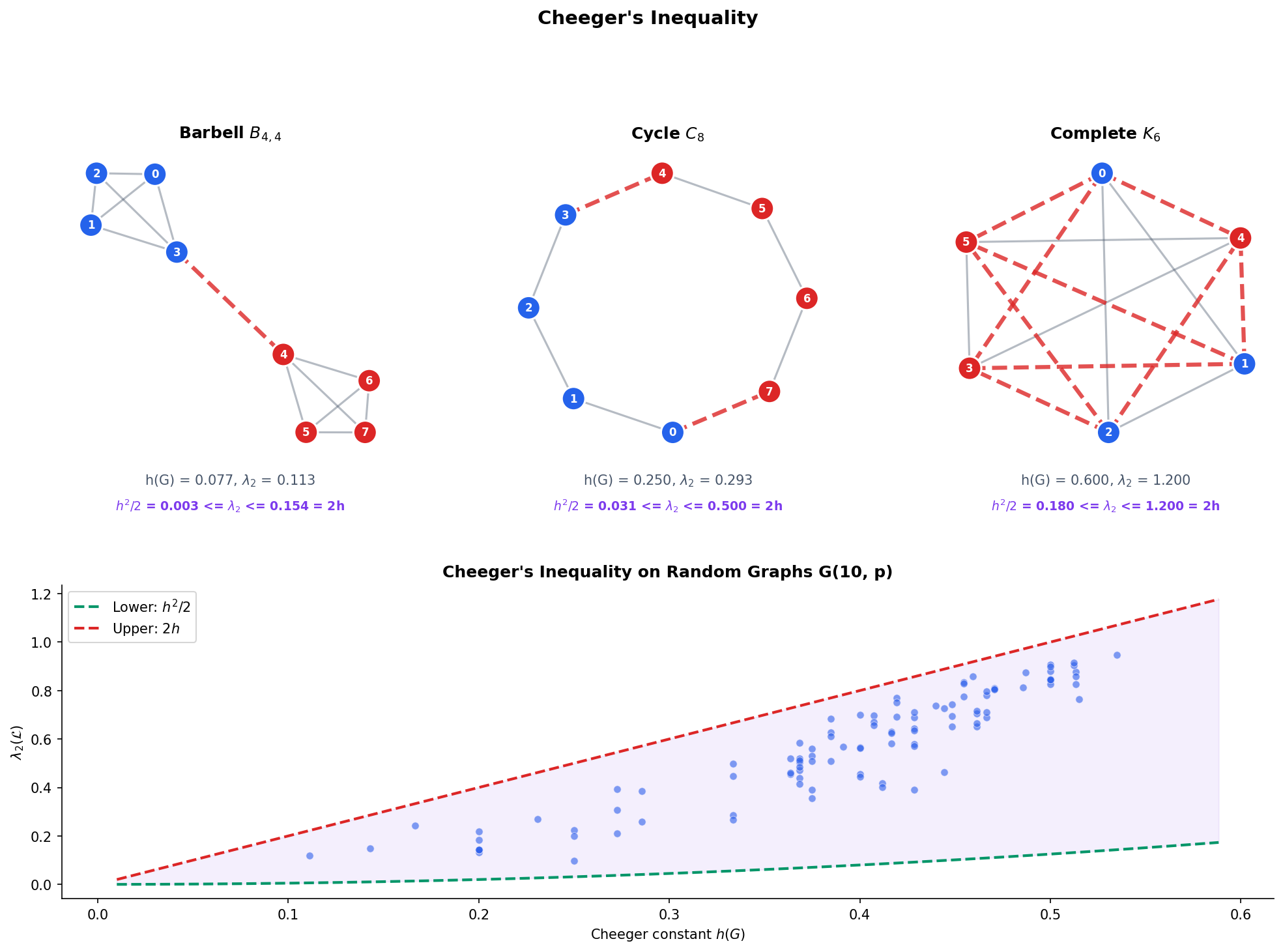
Cheeger’s inequality makes the connection between algebra and combinatorics precise: , where is the Cheeger constant measuring the graph’s combinatorial bottleneck.
Spectral clustering exploits this theory: embed vertices into the eigenspace of the Laplacian, then cluster in the embedding. Points that are non-linearly separable in the original space become linearly separable in the spectral embedding — the same idea as PCA, but with the Laplacian replacing the covariance matrix.
What we cover:
- Graphs and matrices — adjacency, degree, and Laplacian matrices for named graph families.
- The graph Laplacian — definition, quadratic form, positive semidefiniteness, and the zero eigenvalue.
- Spectral properties — eigenvalue ordering, connectivity, the Fiedler value and vector.
- The normalized Laplacian — connection to random walks and transition matrices.
- Cheeger’s inequality — the spectral gap bounds the combinatorial bottleneck.
- Spectral clustering — from similarity graphs to Laplacian eigenmaps to -means.
- Connections to ML — GNNs as Laplacian smoothing, graph signal processing.
- Computational notes — practical implementations in Python.
Graphs, Adjacency Matrices, and the Degree Matrix
We work with undirected, weighted graphs throughout. An undirected graph is the natural setting for the Laplacian: the resulting matrix is symmetric, which is exactly what the Spectral Theorem requires.
Definition 1 (Graph (Undirected, Weighted)).
An undirected weighted graph consists of:
- A finite vertex set ,
- An edge set of unordered pairs,
- A weight function assigning a positive weight to each edge.
For unweighted graphs, for all .
Definition 2 (Adjacency Matrix).
The adjacency matrix of is defined by:
Since is undirected, is symmetric: .
Definition 3 (Degree Matrix).
The degree matrix is the diagonal matrix with entries:
where is the degree (or weighted degree) of vertex — the sum of all edge weights incident to .
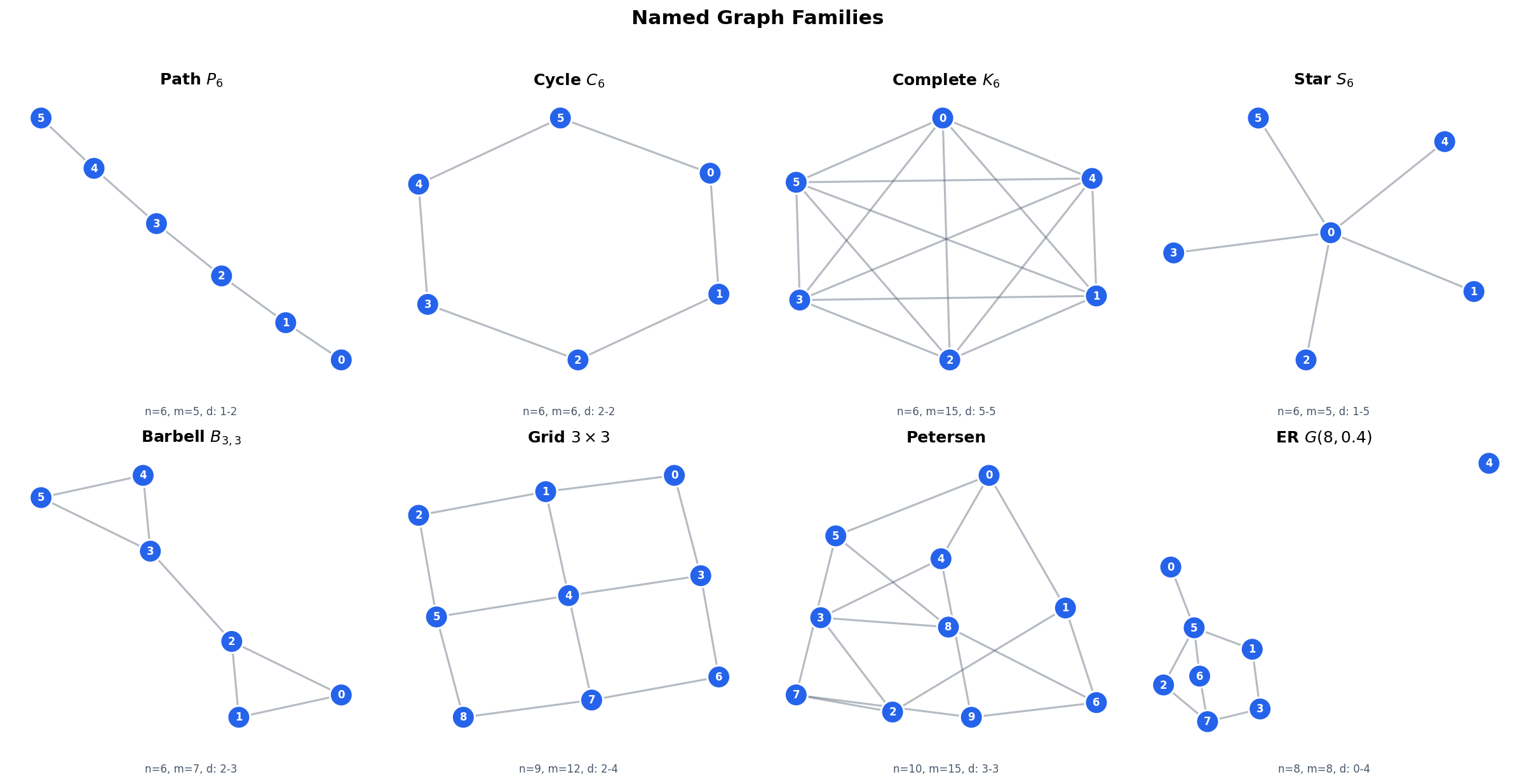
Concrete examples. The topology of a graph shapes its matrix representations. Here are the standard families we will use throughout:
- Path : vertices in a line. is tridiagonal. Each interior vertex has degree 2; endpoints have degree 1.
- Cycle : with the endpoints connected. is tridiagonal plus corner entries. Every vertex has degree 2 (a -regular graph).
- Complete graph : every pair connected. . Every vertex has degree .
- Star : one hub connected to leaves. The hub has degree ; every leaf has degree 1.
- Barbell: two cliques joined by a single bridge edge. This is the canonical bottleneck graph.
- Grid : vertices on a lattice. Interior vertices have degree 4; edges have degree 3; corners have degree 2.
The Graph Laplacian
Definition 4 (Graph Laplacian (Unnormalized)).
The (unnormalized) graph Laplacian of is the matrix:
Equivalently, the entries of are:
Every row and every column of sums to zero: .
The Laplacian looks like a minor rearrangement of , but the sign flip on the off-diagonal entries is what makes it positive semidefinite. The key insight is the quadratic form.
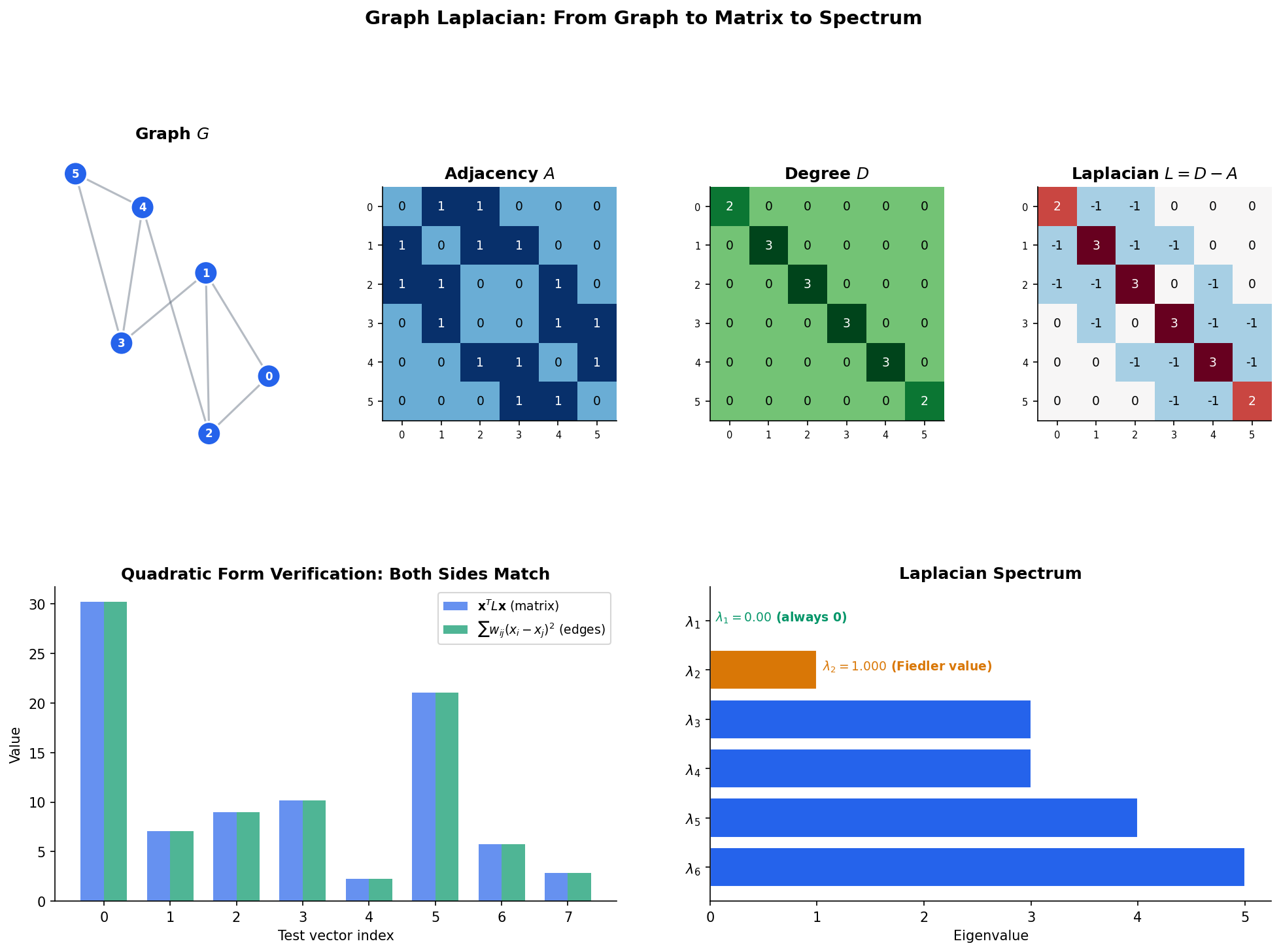
Theorem 1 (Laplacian Quadratic Form).
For any vector :
The quadratic form measures the total variation of the signal across the edges of the graph. A signal that is constant on each connected component has zero variation; a signal that differs wildly across edges has large variation. This is the Dirichlet energy of on .
Proof.
We expand directly:
The first term is . The second is (the factor of 2 because each edge is counted twice in the double sum).
Meanwhile, (each edge contributes from vertex and from vertex ).
Combining:
∎
Theorem 2 (Positive Semidefiniteness of L).
The graph Laplacian is positive semidefinite: for all . Moreover, , so is always an eigenvalue with eigenvector .
Proof.
From Theorem 1, since each term is non-negative (weights are positive, squares are non-negative). This is the definition of positive semidefiniteness.
For the zero eigenvalue: , so .
∎
Remark (Graph Laplacian as Discrete Laplace Operator).
The graph Laplacian is the discrete analog of the continuous Laplace operator . For a function defined on a manifold, measures how much deviates from the average of over a small neighborhood of . Similarly, measures how much deviates from its neighbors’ values. This connection deepens in the Differential Geometry track, where the Laplace–Beltrami operator on Riemannian manifolds generalizes both.
import numpy as np

# Laplacian construction from an adjacency matrix
A = np.array([[0,1,1,0],[1,0,1,1],[1,1,0,0],[0,1,0,0]], dtype=float)
D = np.diag(A.sum(axis=1))
L = D - A

print(f"L = D - A =\n{L}")
# [[ 2. -1. -1.  0.]
#  [-1.  3. -1. -1.]
#  [-1. -1.  2.  0.]
# [ 0. -1. 0. 1.]]Spectral Properties of the Laplacian
Since is real symmetric and PSD, the Spectral Theorem guarantees that its eigenvalues are real and non-negative. We order them:
The first eigenvalue is always (with eigenvector ). The central question is: what does the rest of the spectrum tell us about the graph?
Theorem 3 (Zero Eigenvalue Multiplicity = Number of Connected Components).
The multiplicity of as an eigenvalue of equals the number of connected components of .
Proof.
We characterize the null space of . A vector satisfies if and only if (since is PSD, ). By the quadratic form (Theorem 1):
Since every term is non-negative and , each term must vanish: for every edge . By transitivity along paths, for every pair of vertices in the same connected component.
Therefore if and only if is constant on each connected component. If has connected components , then where is the indicator vector of component . These are linearly independent, so .
∎Corollary 1 (Disconnected Graphs Have λ₂ = 0).
is connected if and only if . Equivalently, is disconnected if and only if .
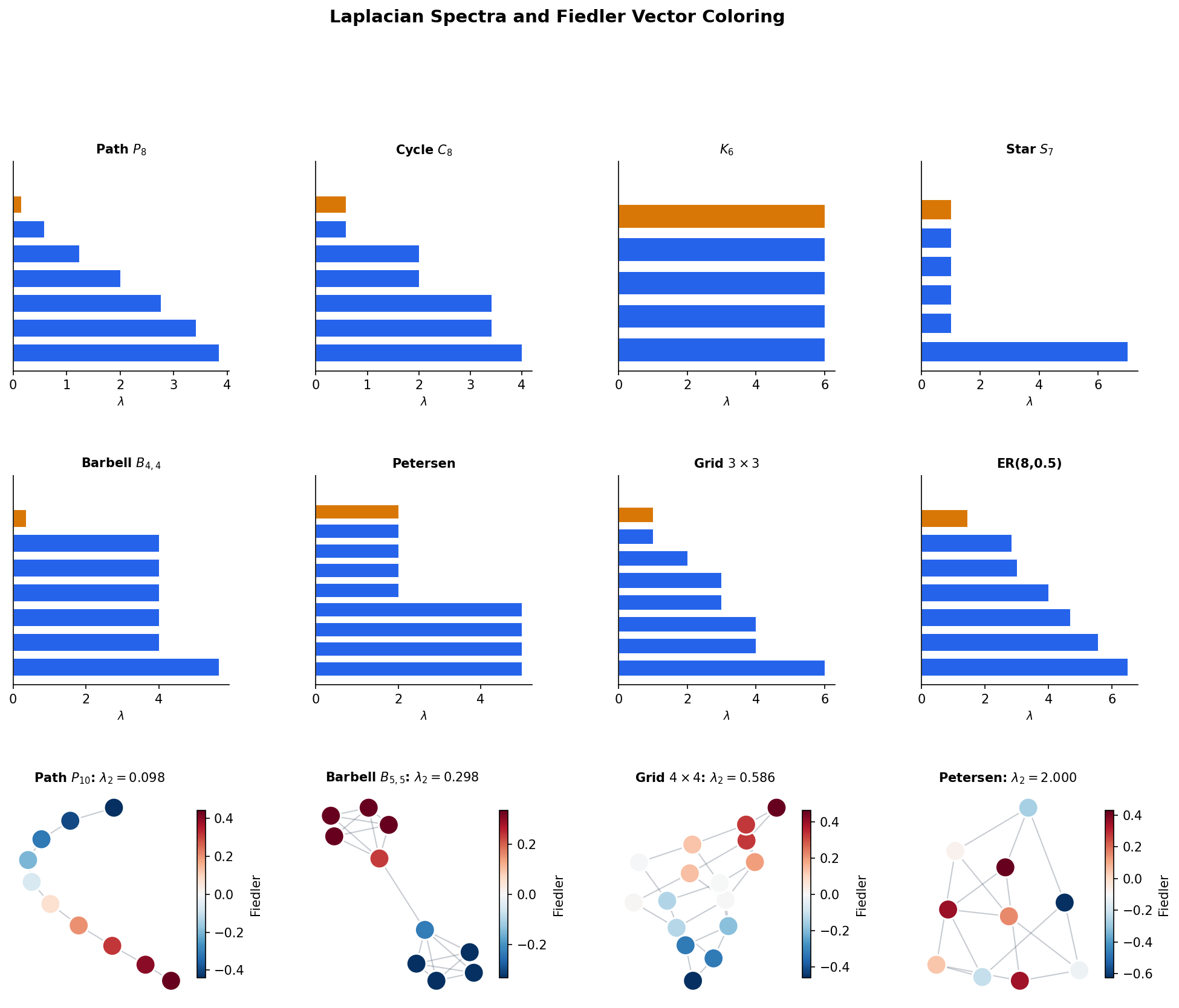
Definition 7 (Algebraic Connectivity (Fiedler Value)).
The algebraic connectivity of a connected graph is the second-smallest eigenvalue , also called the Fiedler value (after Miroslav Fiedler, who introduced it in 1973). The corresponding eigenvector is the Fiedler vector.
The Fiedler value is a spectral measure of “how connected” the graph is. A large means the graph is well-connected with no bottleneck; a small means there is a narrow bridge that nearly disconnects the graph.
Theorem 4 (Fiedler's Theorem (Spectral Bipartitioning)).
For a connected graph , the Fiedler vector provides a near-optimal bipartition. Specifically, the partition , approximates the minimum ratio cut.
The Fiedler value has the variational characterization:
This is the Courant–Fischer characterization from the Spectral Theorem applied to .
Proof.
The variational characterization follows directly from the Courant–Fischer theorem (see Spectral Theorem, Theorem 2): the -th eigenvalue of a symmetric matrix equals the min-max of its Rayleigh quotient. For , we minimize over vectors orthogonal to the first eigenvector .
For the bipartitioning claim: the discrete optimization problem “find minimizing ” is NP-hard. Relaxing the discrete constraint (indicator vectors ) to the continuous constraint (, , ) yields exactly the Fiedler value problem. The Fiedler vector is the solution to this relaxation, and rounding its entries by sign gives a partition that approximates the discrete optimum. This is a convex relaxation of the combinatorial problem.
∎Corollary 2 (Complete Graph Spectrum).
The complete graph has Laplacian eigenvalues (multiplicity 1) and (multiplicity ). Its algebraic connectivity is , the maximum possible for any graph on vertices — is as well-connected as a graph can be.
Proposition 1 (Spectra of Named Graphs).
The Laplacian eigenvalues of standard graph families have closed-form expressions:
- Path : for .
- Cycle : for .
- Star : , , .
Proposition 2 (Laplacian of d-regular Graphs).
If is -regular (every vertex has degree ), then and the Laplacian eigenvalues are , where are the eigenvalues of .
Proof.
Since , we have . If , then . The eigenvalues of are , sorted in ascending order (since is the largest adjacency eigenvalue with eigenvector , giving ).
∎
# Eigendecomposition of the Laplacian
eigenvalues, eigenvectors = np.linalg.eigh(L)
print(f"Eigenvalues: {eigenvalues.round(4)}")
print(f"Fiedler value λ₂ = {eigenvalues[1]:.4f}")
print(f"Fiedler vector v₂ = {eigenvectors[:, 1].round(4)}")The Normalized Laplacian
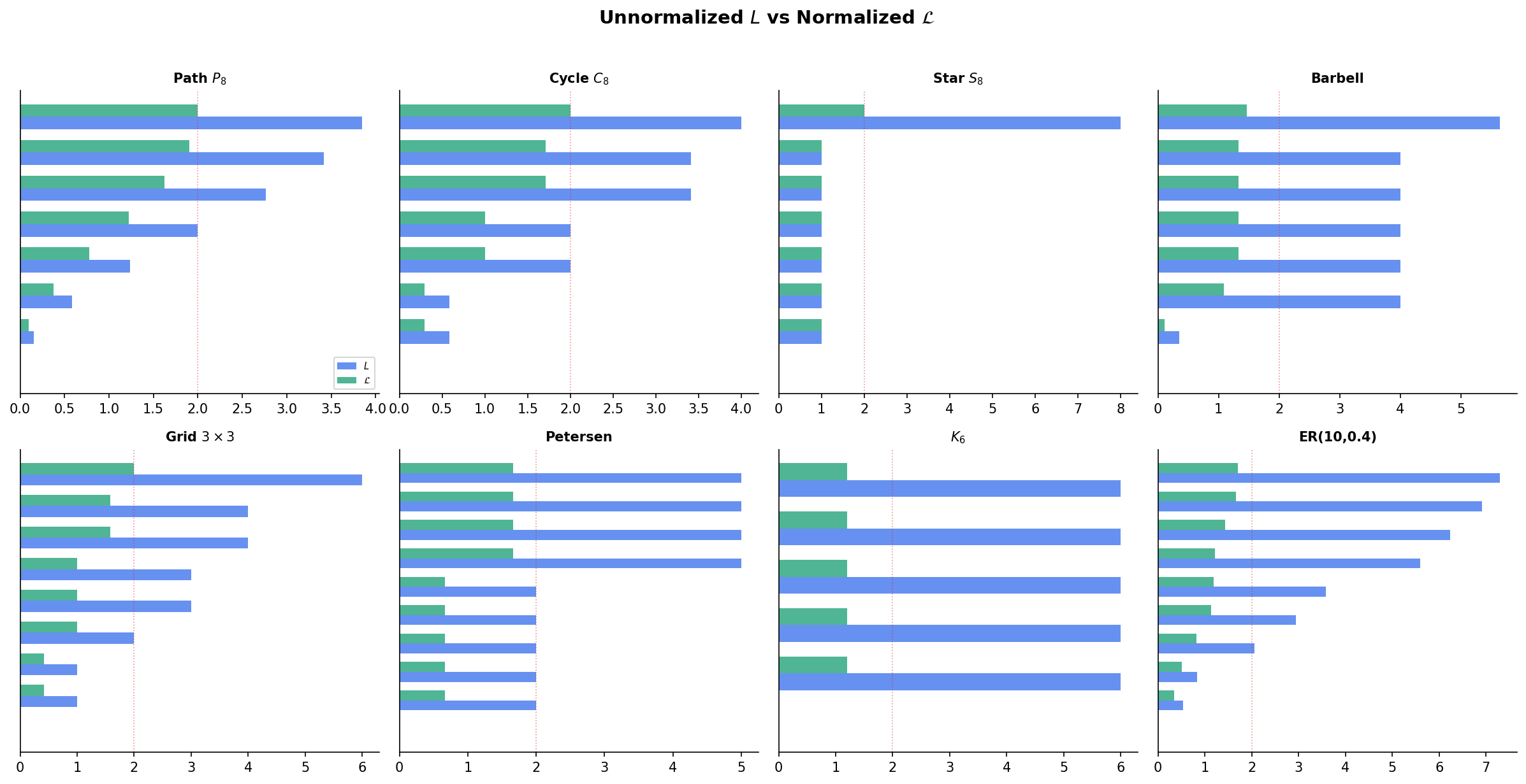
The unnormalized Laplacian treats all vertices equally, regardless of degree. For graphs with heterogeneous degree distributions, the normalized Laplacian accounts for the local connectivity of each vertex.
Definition 5 (Normalized Laplacian).
The symmetric normalized Laplacian is:
where is the diagonal matrix with entries (defined only for vertices with ).
Definition 6 (Random Walk Laplacian).
The random walk Laplacian is:
where is the transition matrix of the random walk on : is the probability of stepping from vertex to vertex .
The three Laplacians are closely related. If , then , so and share eigenvalues. The eigenvectors differ by the transformation .
Theorem 5 (Normalized Laplacian Eigenvalue Range).
All eigenvalues of lie in : .
Proof.
The smallest eigenvalue is with eigenvector (verify: ).
For the upper bound, let be any eigenvector with . Then:
Setting , we have . Using the Cauchy–Schwarz inequality and the constraint that row sums of are bounded, one can show , giving .
More precisely: . By AM-GM, , and (since ). Therefore and .
∎Theorem 7 (Bipartiteness and λₙ = 2).
if and only if has a bipartite connected component. Equivalently, the largest normalized Laplacian eigenvalue equals 2 precisely when the graph contains an odd-cycle-free component.
Proof.
Suppose is bipartite with vertex partition . Define by for and for . Then because every edge connects to , so the sign flips perfectly.
If , then the corresponding eigenvector satisfies , which forces . This means every edge contributes maximally negative correlation: for each edge , and have opposite signs. This is precisely the bipartition condition.
∎Connection to entropy. The random walk on has stationary distribution where is the total edge weight. The Shannon entropy of is . For a -regular graph, is uniform and — the maximum possible entropy. The spectral gap governs how quickly the walk’s distribution converges to , i.e., how fast entropy increases toward equilibrium.
# Normalized Laplacian construction
D_inv_sqrt = np.diag(1.0 / np.sqrt(np.where(d > 0, d, 1)))
L_norm = D_inv_sqrt @ L @ D_inv_sqrt  # = I - D^{-1/2} A D^{-1/2}

eigenvalues_norm = np.linalg.eigh(L_norm)[0]
print(f"Normalized eigenvalues: {eigenvalues_norm.round(4)}")
print(f"All in [0, 2]: {np.all(eigenvalues_norm >= -1e-10) and np.all(eigenvalues_norm <= 2 + 1e-10)}")
Cheeger’s Inequality
The Fiedler value is an algebraic quantity. The Cheeger constant is a combinatorial quantity. Cheeger’s inequality links them, providing a bridge between linear algebra and graph theory.
Definition 8 (Cheeger Constant (Isoperimetric Number)).
The Cheeger constant (or isoperimetric number) of a graph is:
where is the total weight of edges crossing the cut, and is the volume of (the sum of degrees in ).
The Cheeger constant measures the graph’s worst bottleneck: the smallest ratio of “edges crossing a cut” to “the smaller side’s connectivity.” A large means every cut has many crossing edges relative to the smaller side — the graph is well-connected everywhere. A small means there is a narrow bridge.
Theorem 6 (Cheeger's Inequality).
For any graph :
The spectral gap of the normalized Laplacian is sandwiched between and .
Proof.
Easy direction (). We exhibit a test vector that achieves a small Rayleigh quotient.
Let be the subset achieving the Cheeger constant: with . Define the test vector by:
Then is orthogonal to (the first eigenvector of ), and the Rayleigh quotient of gives:
The numerator is and the denominator is . Working through the algebra:
Hard direction () — sketch. This is the deeper inequality. The idea is: given the Fiedler vector , construct a threshold cut by sorting vertices by and sweeping a threshold. By a careful Cauchy–Schwarz argument, the best threshold cut achieves , which gives and hence . The full proof uses the co-area formula on graphs and can be found in Chung (1997), Chapter 2.
∎Interpretation. Cheeger’s inequality says that the spectral gap is a faithful proxy for the combinatorial bottleneck:
- Large large every cut crosses many edges the graph is an expander (the subject of Expander Graphs).
- Small small there exists a narrow bottleneck the graph is nearly disconnected.
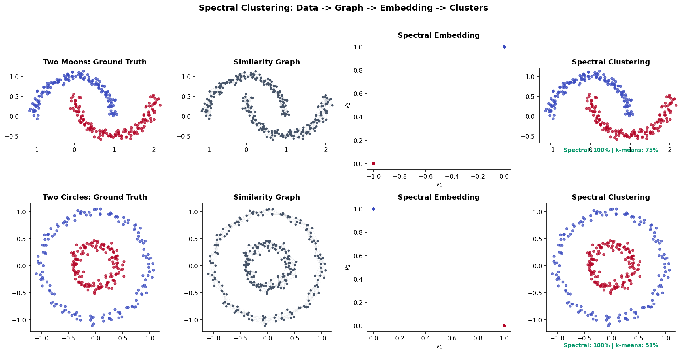
Spectral Clustering
Spectral clustering is the most celebrated application of graph Laplacian theory in machine learning. The idea: transform data using the eigenvectors of a graph Laplacian, then cluster in the transformed space. Points that are non-linearly separable in the original space become linearly separable in the spectral embedding — a phenomenon that standard -means cannot achieve.
Remark (Why 'Spectral' in Spectral Clustering).
The word “spectral” comes from functional analysis, where the set of eigenvalues of an operator is called its spectrum. Spectral clustering uses the eigenvalues and eigenvectors of the graph Laplacian — its spectrum — to find clusters.
The Algorithm
Unnormalized spectral clustering (Laplacian eigenmaps + -means):
- Build a similarity graph. Given data points , construct a -nearest-neighbor graph or -ball graph. Weight edges with the Gaussian kernel:
where is typically set to the median pairwise distance.
-
Compute the Laplacian. Form (unnormalized) or (normalized).
-
Embed. Compute the smallest eigenvectors of (or ). Form the embedding matrix whose columns are these eigenvectors. Each row of is a point in .
-
Cluster. Run -means on the rows of .
Normalized variants (preferred in practice):
- Shi–Malik (2000): Use eigenvectors. Equivalent to normalizing the rows of before -means.
- Ng–Jordan–Weiss (2001): Use eigenvectors, then normalize each row to unit length before -means.
Why It Works
Consider a graph with ideal clusters — cliques with no edges between them. The Laplacian is block diagonal:
Each block has a zero eigenvalue with eigenvector . The bottom eigenvectors of are exactly the indicator vectors of the clusters. The rows of are one-hot vectors, so -means trivially separates them.
When the clusters are not perfectly separated — when there are a few edges between them — the eigenvectors are perturbed versions of the ideal indicators. The perturbation is small when the inter-cluster edges are few (relative to intra-cluster edges), and -means still succeeds.
This is why spectral clustering handles non-convex clusters that -means in the original space cannot: the Laplacian embedding transforms the data from Euclidean proximity (which fails for non-convex shapes) to graph connectivity (which captures the manifold structure).
from sklearn.cluster import SpectralClustering
from sklearn.datasets import make_moons

# Two moons: non-convex clusters that k-means cannot separate
X, y = make_moons(200, noise=0.06, random_state=42)

sc = SpectralClustering(
    n_clusters=2,
    affinity='nearest_neighbors',
    n_neighbors=10,
    random_state=42
)
labels = sc.fit_predict(X)
accuracy = max(np.mean(labels == y), np.mean(1 - labels == y))
print(f"Spectral clustering accuracy: {accuracy:.1%}") # ~100%Connections to Machine Learning
Graph Signal Processing
A graph signal is a function that assigns a real value to each vertex. The eigenvectors of the Laplacian form an orthonormal basis — the graph Fourier basis — and the graph Fourier transform of is:
where is the matrix of Laplacian eigenvectors. Low-eigenvalue components correspond to smooth signals (slowly varying across edges); high-eigenvalue components correspond to rough signals (rapidly varying). Filtering in the spectral domain — zeroing out high-frequency components — amounts to smoothing the signal on the graph.
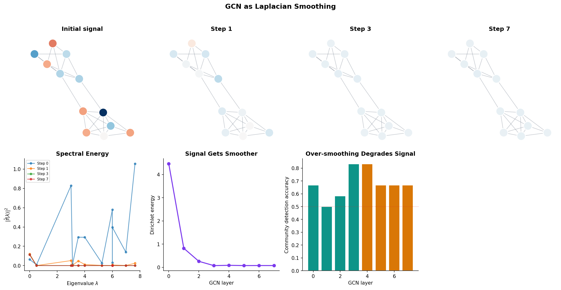
GCNs as Laplacian Smoothing
The Graph Convolutional Network (GCN) of Kipf & Welling (2017) performs the update:
where is the adjacency matrix with added self-loops and is its degree matrix. The matrix is one minus the normalized Laplacian of the self-loop-augmented graph. This means each GCN layer smooths the node features: every node’s representation is replaced by a weighted average of itself and its neighbors.
Remark (GCN as Laplacian Smoothing).
The renormalization trick avoids the need to explicitly add a skip connection. Without self-loops, averages over neighbors only; with self-loops, averages over neighbors and the node itself. This is a low-pass filter on the graph: it amplifies low-frequency (smooth) components and attenuates high-frequency (rough) components. Stacking too many GCN layers causes over-smoothing — all node features converge to the same value, dominated by the eigenvector for .
Message Passing & GNNs develops this connection further, showing how message-passing neural networks generalize GCNs and how the Laplacian spectrum determines what a GNN can and cannot learn.
import torch

# Single GCN layer: H' = σ(D̃^{-1/2} Ã D̃^{-1/2} H W)
A_tilde = A + torch.eye(n)                  # Add self-loops
D_tilde = torch.diag(A_tilde.sum(dim=1))
D_inv_sqrt = torch.diag(1.0 / torch.sqrt(D_tilde.diagonal()))
S = D_inv_sqrt @ A_tilde @ D_inv_sqrt       # Normalized adjacency

H = torch.randn(n, 16)                      # Node features
W = torch.randn(16, 8)                       # Learnable weights
H_next = torch.relu(S @ H @ W)              # One GCN layer
Computational Notes
NumPy / SciPy
import numpy as np
from scipy.sparse import csr_matrix
from scipy.sparse.csgraph import laplacian

# Dense Laplacian
A = np.array([[0,1,1,0],[1,0,1,1],[1,1,0,0],[0,1,0,0]], dtype=float)
D = np.diag(A.sum(axis=1))
L = D - A

# Eigendecomposition (use eigh for symmetric matrices — faster and more stable)
eigenvalues, eigenvectors = np.linalg.eigh(L)
fiedler_value = eigenvalues[1]
fiedler_vector = eigenvectors[:, 1]

# Sparse Laplacian (for large graphs)
A_sp = csr_matrix(A)
L_sp = laplacian(A_sp)
NetworkX
import networkx as nx

G = nx.from_numpy_array(A)
print(f"Spectrum: {np.sort(nx.laplacian_spectrum(G)).round(4)}")
print(f"Algebraic connectivity: {nx.algebraic_connectivity(G):.4f}")
print(f"Fiedler vector: {nx.fiedler_vector(G).round(4)}")
scikit-learn
from sklearn.cluster import SpectralClustering

sc = SpectralClustering(
    n_clusters=2,
    affinity='nearest_neighbors',
    n_neighbors=10,
    random_state=42
)
labels = sc.fit_predict(X)
Practical tips:
- Always use
np.linalg.eigh(noteig) for symmetric matrices — it is faster, more numerically stable, and guarantees real eigenvalues. - Threshold near-zero eigenvalues: treat as zero when counting connected components.
- For large sparse graphs, use
scipy.sparse.linalg.eigsh(L, k=3, which='SM')to compute only the smallest eigenvalues. - Set the Gaussian kernel bandwidth to the median pairwise distance — a robust default.
Connections & Further Reading
| Topic | Connection |
|---|---|
| The Spectral Theorem | The graph Laplacian is real symmetric. The Spectral Theorem guarantees a complete orthonormal eigenbasis — the foundation of spectral graph theory. The Courant–Fischer theorem underlies the Fiedler value characterization and Cheeger’s inequality. |
| Shannon Entropy & Mutual Information | The entropy of the random walk stationary distribution measures graph regularity. Regular graphs have uniform and maximum entropy . The spectral gap governs the mixing rate. |
| PCA & Low-Rank Approximation | Spectral clustering uses the bottom eigenvectors of the Laplacian as an embedding, analogous to PCA using the top eigenvectors of the covariance matrix. Both are eigenmap embeddings: PCA preserves variance, spectral clustering preserves graph connectivity. |
| Convex Analysis | The quadratic form is convex. Spectral clustering relaxes the NP-hard normalized cut to a continuous eigenvalue problem — a convex relaxation. |
| Random Walks & Mixing | The transition matrix has eigenvalues , and the spectral gap controls mixing time — how quickly the walk’s distribution converges to the stationary distribution. |
| Expander Graphs | Expander Graphs studies the graphs that maximize connectivity at fixed sparsity. The spectral gap — bounded below by Cheeger’s inequality — is the defining quantity: expanders have spectral gap bounded away from zero. |
| Message Passing & GNNs | GCN message passing is Laplacian smoothing. Over-smoothing occurs when too many layers act as a low-pass filter, collapsing all node features toward the dominant eigenvector. |
Key Notation
| Symbol | Meaning |
|---|---|
| Unnormalized graph Laplacian | |
| Normalized Laplacian | |
| Random walk Laplacian | |
| Random walk transition matrix | |
| Fiedler value (algebraic connectivity) | |
| Fiedler vector | |
| Cheeger constant | |
| Volume of vertex set |
Connections
- The graph Laplacian is a real symmetric matrix. The Spectral Theorem guarantees it has a complete orthonormal eigenbasis with real eigenvalues — the foundation of every result in spectral graph theory. spectral-theorem
- The entropy of a random walk's stationary distribution measures graph regularity. On a d-regular graph, the stationary distribution is uniform with maximum entropy log(n). The spectral gap governs how quickly the walk's distribution converges to stationarity — how fast entropy increases. shannon-entropy
- The Laplacian quadratic form x^T L x = sum_{(i,j)} w_{ij}(x_i - x_j)^2 is a convex function whose minimization (subject to constraints) yields the Fiedler vector. Graph cuts are combinatorial optimization problems relaxed to spectral problems via convex relaxation. convex-analysis
- Spectral clustering uses the bottom eigenvectors of the Laplacian as a low-dimensional embedding — analogous to PCA using the top eigenvectors of the covariance matrix. Both are instances of eigenmap embeddings that preserve specific notions of structure. pca-low-rank
References & Further Reading
- book Spectral Graph Theory — Chung (1997) The foundational text — covers the normalized Laplacian, Cheeger's inequality, and connections to random walks
- book Algebraic Graph Theory — Godsil & Royle (2001) Chapters 8-9 cover the adjacency and Laplacian spectra with algebraic rigor
- paper A Tutorial on Spectral Clustering — von Luxburg (2007) The standard reference for spectral clustering — bridges graph Laplacian theory to machine learning practice
- paper Semi-Supervised Classification with Graph Convolutional Networks — Kipf & Welling (2017) GCN = renormalized Laplacian smoothing — the paper that made graph Laplacians central to deep learning
- paper The Laplacian Spectrum of Graphs — Mohar (1991) Survey of Laplacian eigenvalue bounds and their combinatorial interpretations
- book Graph Signal Processing: Overview, Challenges, and Applications — Ortega, Frossard, Kovačević, Moura & Vandergheynst (2018) Graph Fourier transform = eigenvector expansion of the Laplacian