Stochastic-Gradient MCMC

1. Overview & Motivation

The point of bayesian-neural-networks was to put a posterior on the weights of a deep network. Five of the eight methods we developed there were either approximations to the posterior (Laplace, MC-dropout, deep ensembles) or local tricks (calibration, NNGP/NTK). Two were exact-in-the-limit posterior samplers: stochastic-gradient Langevin dynamics (SGLD, BNN §6) and stochastic-gradient Hamiltonian Monte Carlo (SGHMC, BNN §7). Both arrived as recipes — write down an update rule, calibrate the noise, run the chain. The recipes work, but BNN didn’t tell us why they work.

This topic is the answer. The throughline is that SGLD and SGHMC are not two unrelated tricks but two instantiations of a single object: a stochastic differential equation whose stationary distribution is the posterior we want to sample. Once we accept that frame, three things follow at once. The asymptotic exactness of SGLD becomes a Fokker–Planck calculation. The momentum trick in SGHMC becomes the underdamped version of the same SDE. And every other SG-MCMC method that ever shipped — Riemann-manifold variants, control-variate variants, thermostat methods — drops out of a single skew-symmetric matrix decomposition due to Ma, Chen, and Fox (2015).

That’s the headline. Below it sit four secondary questions this topic resolves:

• What does the mini-batch gradient cost us? SGLD’s update rule replaces the full-data gradient with a mini-batch estimate. This is the only reason the method scales, but it injects extra noise into the SDE. Vollmer, Zygalakis, and Teh (2016) gave the finite-sample bias bound: under regularity, $\mathbb{E}[\phi(\theta_T)] - \pi(\phi) = O(\eta + B^{-1})$. We work that bound out and show what it means in practice.
• When does SGHMC actually beat SGLD? The momentum extension is more expensive per step. We characterize the friction–noise trade-off (Chen, Fox, and Guestrin 2014) and pin down the regime where SGHMC’s faster mixing pays for its higher cost — anisotropic posteriors with badly-conditioned curvature.
• What about hierarchical models like Neal’s funnel? The same funnel that motivated probabilistic-programming’s non-centered reparameterization breaks SGLD and SGHMC alike, for the same geometric reason. The fix is to replace the Euclidean metric with the Fisher information — Riemann-manifold SG-MCMC (Patterson and Teh 2013; Ma, Chen, and Fox 2015). We derive the correction term and demonstrate the speedup.
• When should I reach for SG-MCMC over NUTS? Closed answer at the end of the topic, with a head-to-head ESS-per-second comparison on a Bayesian logistic regression as $N$ grows from $500$ to $50{,}000$. NUTS dominates at small $N$; SG-MCMC dominates once full-batch gradients become the bottleneck.

1.1 What we cover

§§2–4 set up the SDE machinery: the complete-recipe framework that organizes the rest of the topic, an Itô-SDE primer (self-contained because formalcalculus has not yet published its SDE topic), and the Fokker–Planck calculation that proves a given SDE has the posterior as its stationary distribution. §§5–7 develop overdamped Langevin → SGLD and underdamped Langevin → SGHMC, with the stationary-distribution proofs reused from §4. §§8–9 quantify the price of mini-batching and present the strategies that buy bias back at controlled cost. §10 extends the framework to Riemann manifolds and demonstrates on Neal’s funnel. §11 ships the implementation details (per-method step functions, hyperparameter recipes, ESS/IAT diagnostics) as the foundations-track Computational Notes section. §12 puts SG-MCMC head-to-head with NUTS and articulates when each wins. §13 collects connections and forward pointers.

1.2 Prerequisites

The reader is expected to have read bayesian-neural-networks at least through §7 (so the SGLD and SGHMC update rules are familiar as recipes, even if the underlying SDE theory is not). probabilistic-programming §§4–5 (NUTS, the centered/non-centered funnel) is helpful for §12 and the §10 Neal’s-funnel demo but is not strictly required. From the sister sites we lean on formalstatistics’s bayesian-computation-and-mcmc (the deep prerequisite — what makes an MCMC method correct and how to read mixing diagnostics) and basic familiarity with stochastic processes (Brownian motion, the difference between an ODE and an SDE). Itô calculus itself is not assumed; §3 covers the minimum.

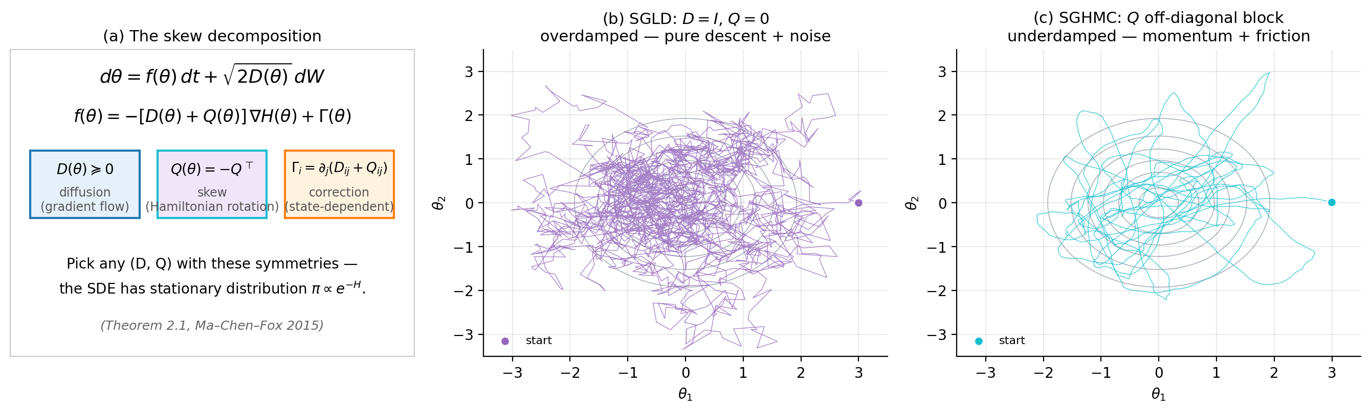
2. The complete-recipe lens

Before we develop SGLD or SGHMC in detail, we need to understand what they have in common — and what every other SG-MCMC method that has ever shipped also has in common. The unifying object is a single SDE template parametrized by two matrix-valued functions: a positive semi-definite diffusion $D(\theta)$ and a skew-symmetric drift modifier $Q(\theta)$. Different choices of $(D, Q)$ yield SGLD, SGHMC, RMHMC, RSGLD, thermostats, and more, with the same proof of stationarity covering all of them. The result is due to Ma, Chen, and Fox (2015), and we lean on it heavily for the rest of the topic.

2.1 The general posterior-targeting SDE template

Let $\pi(\theta) \propto \exp(-H(\theta))$ be the target distribution we want to sample. For the Bayesian posterior, $H(\theta) = -\log p(\theta) - \sum_{i=1}^N \log p(y_i \mid \theta)$ — the negative log-prior plus the sum of negative log-likelihoods over the dataset, up to an additive constant. We will call $H$ the energy of the target, borrowing the physics convention; statisticians sometimes call it the negative log-posterior. Either way, $\nabla H = -\nabla \log \pi$ is the quantity that drives the dynamics.

We are looking for an Itô SDE of the form

$$d\theta_t = f(\theta_t)\, dt + \sqrt{2\, D(\theta_t)}\, dW_t \qquad \qquad (2.1)$$

whose stationary distribution is exactly $\pi$. Here $W_t$ is standard Brownian motion in $\mathbb{R}^d$ (we develop this object from scratch in §3), $D(\theta) \in \mathbb{R}^{d \times d}$ is positive semi-definite at every point, and $\sqrt{2D}$ is any matrix square root (e.g., a Cholesky factor — the choice does not affect the law of $\theta_t$, only its sample path). The drift $f(\theta) \in \mathbb{R}^d$ is what we are solving for.

The continuous-time SDE in (2.1) is the object whose stationarity we will prove. SGLD and SGHMC are what we get when we discretize (2.1) with Euler–Maruyama and replace $\nabla H$ with a mini-batch estimator. We work that side of the story out in §§5–7.

2.2 The Ma–Chen–Fox skew decomposition

Here is the headline.

The proof is a Fokker–Planck calculation. We carry it out in §4.3 once we have the Fokker–Planck operator in hand; the argument is short but it requires the machinery from §3 and §4 to make any sense, so we defer it. For now, the takeaway is that the criterion for stationarity is purely algebraic: pick a $D$ and a $Q$ with the stated symmetry, compute $\Gamma$ by differentiating their entries, and you have an SDE with stationary distribution $\pi$.

A few things deserve immediate comment. The $-D \nabla H$ term is the gradient-flow part: it pulls $\theta$ toward high-density regions, much like ordinary gradient descent on $H$. The $\sqrt{2D}\, dW_t$ term is the Brownian noise that prevents collapse to the mode and makes the dynamics ergodic. The $-Q \nabla H$ term and the correction $\Gamma$ together produce the Hamiltonian part of the dynamics — the rotational, momentum-like behavior we will see in SGHMC. When $Q = 0$, the dynamics reduce to gradient flow plus noise (this is SGLD). When $Q \neq 0$, we get rotation around level sets of $H$, which mixes much faster on anisotropic targets but costs more per step.

Skew-symmetry of $Q$ is what makes the theorem work — a symmetric $Q$ would break stationarity. Why? In the Fokker–Planck calculation (§4.3), $Q$ enters via a divergence term that integrates to zero precisely when $Q^\top = -Q$. We give the calculation in §4 once we have the Fokker–Planck operator; for now, take the skew condition as a mathematical requirement that emerges from the proof and not as a modeling choice.

2.3 Three instantiations

The whole topic is, in a real sense, a tour of three choices of $(D, Q)$.

SGLD. Take $D = I$, the $d \times d$ identity, and $Q = 0$. Then $\Gamma = 0$ (constant matrix entries have zero derivative), and $f(\theta) = -\nabla H(\theta)$. The SDE is

$$d\theta_t = -\nabla H(\theta_t)\, dt + \sqrt{2}\, dW_t.$$

This is overdamped Langevin dynamics. Discretizing with Euler–Maruyama gives the SGLD update from BNN §6.2. We develop this case in §§5–6.

SGHMC. Now expand the state to $(\theta, r) \in \mathbb{R}^{2d}$ with $r$ playing the role of momentum, and choose

$$D = \begin{pmatrix} 0 & 0 \\ 0 & C \end{pmatrix}, \qquad Q = \begin{pmatrix} 0 & -I \\ I & 0 \end{pmatrix}, \qquad H(\theta, r) = U(\theta) + \tfrac{1}{2} r^\top M^{-1} r,$$

where $C$ is a friction matrix and $M$ is a mass matrix (both positive definite). The marginal of the joint stationary $\pi(\theta, r) \propto \exp(-H(\theta, r))$ over $r$ is exactly the target posterior on $\theta$. The drift in this expanded state space gives the second-order underdamped Langevin dynamics of Chen, Fox, and Guestrin (2014). We develop this case in §7.

RMHMC and RSGLD. Replace the constant $D = I$ in SGLD with a state-dependent $D(\theta) = G(\theta)^{-1}$, where $G(\theta)$ is the Fisher information metric (or any other positive-definite metric on parameter space). The correction term $\Gamma$ becomes nonzero — that’s the famous $\nabla \cdot G^{-1}$ correction in Riemann-manifold methods (Patterson and Teh 2013; Girolami and Calderhead 2011). For the Hamiltonian version, also replace the constant $Q$ in SGHMC with $G(\theta)^{-1}$-blocks. We develop this case in §10.

2.4 What the framework tells us, and what it doesn’t

Theorem 2.1 says that if you can run the SDE exactly, your samples are exactly from $\pi$. It says nothing about what happens when (a) you discretize the SDE into finite-step updates, (b) you replace the full-data gradient with a mini-batch estimator, or (c) you stop the chain after finitely many steps. Each of those introduces a finite-sample bias, and each is the subject of its own section: (a) is the Euler–Maruyama discretization error in §5–7; (b) is the mini-batch noise quantified by Vollmer, Zygalakis, and Teh (2016) in §8; (c) is the mixing-time question we read off chain autocorrelations throughout. The complete recipe gives us the target — the SDE we are trying to discretize. The rest of the topic is about how close to that target we actually land.

Computing chain trajectories…

3. Itô SDE preliminaries

Theorem 2.1 referred to a “stochastic differential equation” without saying what one is. We owe the reader a definition before we use it again. This section gives the minimum needed for the rest of the topic — Brownian motion, the Itô integral, Itô SDEs, Itô’s lemma, and the Euler–Maruyama discretization — and it stops there. A full development belongs in formalcalculus’s eventual stochastic-differential-equations topic; until that ships, what follows is self-contained.

3.1 Brownian motion

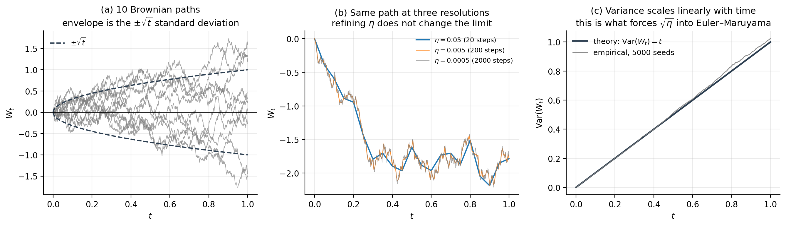
Brownian motion (or Wiener process) is the canonical source of continuous-time noise. A standard $d$-dimensional Brownian motion is a stochastic process $W = (W_t)_{t \geq 0}$ with values in $\mathbb{R}^d$ satisfying four properties: $W_0 = 0$ almost surely; the increments $W_{t+s} - W_t$ are independent of the history $\{W_u : u \leq t\}$ for any $s > 0$; each increment is Gaussian with $W_{t+s} - W_t \sim \mathcal{N}(0, s\, I_d)$ — note the variance $s$, not $s^2$; and the sample paths $t \mapsto W_t$ are continuous with probability one.

Two consequences are worth pulling out. First, the variance scales linearly with elapsed time, $\mathrm{Var}(W_t) = t \cdot I_d$, so the typical magnitude of $W_t$ grows like $\sqrt{t}$. Second, the paths are continuous but nowhere differentiable — Brownian motion has finite quadratic variation but infinite first variation, so the naive notation "$dW_t/dt$" is not a function in the classical sense. This is why we cannot integrate against $W$ as if it were a smooth signal; we need a different integral.

Computing Brownian paths…

3.2 Itô SDEs

Define an Itô SDE in $\mathbb{R}^d$ as

$$dX_t = a(X_t, t)\, dt + b(X_t, t)\, dW_t \qquad \qquad (3.1)$$

with drift $a : \mathbb{R}^d \times \mathbb{R}_+ \to \mathbb{R}^d$, diffusion $b : \mathbb{R}^d \times \mathbb{R}_+ \to \mathbb{R}^{d \times d}$, and $W_t$ a $d$-dimensional standard Brownian motion. Equation (3.1) is shorthand for the integral equation

$$X_t = X_0 + \int_0^t a(X_s, s)\, ds + \int_0^t b(X_s, s)\, dW_s,$$

where the second integral is the Itô integral. The Itô integral is built as a limit of left-endpoint Riemann sums: partition $[0, t]$ into $0 = t_0 < t_1 < \cdots < t_n = t$, form the sum $\sum_k b(X_{t_k}, t_k)(W_{t_{k+1}} - W_{t_k})$, and let the mesh size go to zero. The “left-endpoint” choice — evaluating $b$ at the start of each subinterval, not the midpoint or right end — is what makes Itô integrals martingales: $\mathbb{E}\!\left[\int_0^t b(X_s, s)\, dW_s\right] = 0$, which we will use repeatedly.

Under standard regularity assumptions on $a$ and $b$ (Lipschitz continuity and linear growth), the SDE (3.1) has a unique strong solution given an initial condition $X_0$. We will not prove existence and uniqueness; the SDEs we encounter — Langevin, Hamiltonian Langevin, Riemann-manifold variants — all satisfy the assumptions provided $H \in C^2$ and grows sufficiently fast at infinity.

3.3 Itô’s lemma

Itô’s lemma is the chain rule for SDEs, and we will lean on it twice — once to verify the stationary-distribution claim of Theorem 2.1 (in §4.3), and once again when we set up Riemann-manifold dynamics (§10). The statement is:

The first two terms are what an ordinary chain rule would give. The third term is the Itô correction: it appears because the quadratic variation of $W_t$ is $t$, not zero, so $(dW_t)^2 = dt$ in the Itô calculus and the second-order Taylor term in $\phi$ does not vanish in the limit. We will use the correction in exactly the form that lets us read off the Fokker–Planck operator: applying (3.2) to a smooth test function and taking expectations gives the generator of the SDE, and the divergence theorem then converts the generator into a PDE for the density of $X_t$. We carry this out in §4.

3.4 Euler–Maruyama discretization

Solving an SDE in closed form is rare. Almost everything we run on a computer is an approximation, and the simplest is Euler–Maruyama: pick a step size $\eta > 0$, set $X_n \approx X_{n\eta}$, and update

$$X_{n+1} = X_n + a(X_n, n\eta)\, \eta + b(X_n, n\eta)\, \sqrt{\eta}\, \xi_n, \qquad \xi_n \overset{\text{iid}}{\sim} \mathcal{N}(0, I_d). \qquad \qquad (3.3)$$

The $\sqrt{\eta}$ — not $\eta$ — in front of the noise term is non-negotiable: it is what gives $\sqrt{\eta}\, \xi_n$ the same distribution as the increment $W_{(n+1)\eta} - W_{n\eta}$, namely $\mathcal{N}(0, \eta\, I_d)$. Substitute $\eta$ in its place and the resulting scheme converges to a different (typically wrong) SDE. Every SG-MCMC update in this topic is some flavor of (3.3), so getting this scaling right is the single most important detail in the implementation.

The Euler–Maruyama scheme has strong order $1/2$ — meaning $\mathbb{E}|X_{n} - X_{n\eta}| = O(\sqrt{\eta})$ at fixed final time — and weak order $1$ — meaning $\mathbb{E}\phi(X_n) - \mathbb{E}\phi(X_{n\eta}) = O(\eta)$ for sufficiently smooth $\phi$. The weak order is what matters for MCMC, since we care about expectations against the stationary distribution rather than path accuracy. It is also where the $O(\eta)$ term in the Vollmer–Zygalakis–Teh bias bound (§8) comes from.

3.5 What we need going forward

§4 uses (3.1) and (3.2) to derive the Fokker–Planck equation, then specializes to verify Theorem 2.1. §§5–7 use (3.3) repeatedly: SGLD is Euler–Maruyama on overdamped Langevin, SGHMC is a leapfrog-flavored discretization of underdamped Langevin. §10 reuses Itô’s lemma when the diffusion coefficient becomes state-dependent through a Riemann metric. Nothing in what follows requires SDE theory beyond what we have just assembled.

4. Fokker–Planck and stationary distributions

§3 gave us the Itô SDE as a stochastic process. We now ask the question that the rest of the topic depends on: given an SDE, what is the time-evolution of the density of its solution, and which densities are stationary? The answer is the Fokker–Planck equation. Once we have it, the proof of Theorem 2.1 is two pages of bookkeeping.

4.1 The Fokker–Planck equation

Let $\rho(\theta, t)$ be the density of $X_t$ at time $t$ — i.e., $\mathbb{P}(X_t \in A) = \int_A \rho(\theta, t)\, d\theta$ — for the Itô SDE

$$dX_t = a(X_t)\, dt + \sqrt{2 D(X_t)}\, dW_t,$$

where we have specialized to time-homogeneous coefficients (drift and diffusion depend only on $\theta$, not on $t$) since this is the case relevant to MCMC. We want a PDE for $\rho$.

The derivation is a one-step application of Itô’s lemma. Let $\phi : \mathbb{R}^d \to \mathbb{R}$ be any smooth, compactly supported test function and consider $\mathbb{E}[\phi(X_t)] = \int \phi(\theta)\, \rho(\theta, t)\, d\theta$. Differentiating in $t$ and using Itô’s lemma (Lemma 3.1) on $\phi(X_t)$:

$$\frac{d}{dt} \mathbb{E}[\phi(X_t)] = \mathbb{E}\!\left[\nabla \phi^\top a(X_t) + \mathrm{tr}\!\left(D(X_t)\, \nabla^2 \phi\right)\right] = \int \rho(\theta, t)\!\left[\nabla \phi^\top a + \mathrm{tr}(D\, \nabla^2 \phi)\right] d\theta.$$

Integrating by parts twice — possible because $\phi$ is compactly supported, so all boundary terms vanish — and matching coefficients of $\phi$ gives the Fokker–Planck equation:

$$\partial_t \rho = -\nabla \!\cdot\! (a\, \rho) + \sum_{i,j=1}^d \partial_i \partial_j (D_{ij}\, \rho). \qquad \qquad (4.1)$$

The first term on the right is the drift current — probability mass flowing along the deterministic vector field $a$. The second term is the diffusion current — probability mass spreading out under the noise. The equation is sometimes called the forward Kolmogorov equation; some authors absorb the factor of two and write it for $\sigma = \sqrt{D}$ instead of $D$. Our form, with the $\sqrt{2D}$ in the SDE matching the bare $D$ in (4.1), is the convention that makes Theorem 2.1 read cleanly.

t:0.50α:1.0σ:1.0

(a) p(x, t = 0.50)

(b) σ²(t) → σ²/(2α) = 0.500

4.2 Stationarity, probability currents, and detailed balance

A density $\pi$ is stationary for the SDE if $\partial_t \rho = 0$ when $\rho = \pi$. Setting the right-hand side of (4.1) to zero gives a stationarity condition that is best expressed in terms of the probability current $J : \mathbb{R}^d \to \mathbb{R}^d$ defined by

$$J_i(\theta) = a_i(\theta)\, \rho(\theta) - \sum_{j=1}^d \partial_j \!\bigl[D_{ij}(\theta)\, \rho(\theta)\bigr], \qquad \qquad (4.2)$$

so that (4.1) becomes the conservation-of-mass form $\partial_t \rho = -\nabla \!\cdot\! J$. Stationarity is then equivalent to

$$\nabla \!\cdot\! J(\pi) = 0 \quad \text{everywhere.} \qquad \qquad (4.3)$$

There are two ways for (4.3) to hold. The strong form is detailed balance: $J(\pi) \equiv 0$ pointwise. Detailed balance corresponds to time-reversibility — the chain looks statistically the same run forward or backward — and is what overdamped Langevin / SGLD will satisfy. The weak form is cyclic stationarity: $J(\pi) \neq 0$ but $\nabla \!\cdot\! J(\pi) = 0$, meaning probability mass circulates without accumulating. SGHMC and Riemann-manifold methods generically satisfy the weak form but not the strong one. Both kinds of solution sample from $\pi$ in the long run; the difference matters for asymptotic-variance calculations and for some convergence proofs but not for the basic correctness claim.

4.3 Proof of Theorem 2.1

We can now finish the proof we deferred from §2. Take

$$a(\theta) = -\bigl[D(\theta) + Q(\theta)\bigr] \nabla H(\theta) + \Gamma(\theta), \qquad \Gamma_i = \sum_j \partial_j (D_{ij} + Q_{ij}),$$

with $D \succeq 0$ and $Q^\top = -Q$. We want to show that $\pi(\theta) \propto \exp(-H(\theta))$ satisfies (4.3). The plan is to compute $J(\pi)$ explicitly, observe that it has a clean form, and then verify $\nabla \!\cdot\! J(\pi) = 0$ using the skew condition.

Theorem 2.1 holds, and the entire ledger of SG-MCMC methods — SGLD, SGHMC, RSGLD, RMHMC, thermostat methods — inherits stationarity from this single calculation by choosing different $(D, Q)$.

4.4 What this gives us

Two operational consequences carry through the rest of the topic. First, exact-in-the-limit stationarity is automatic for any scheme that discretizes a Theorem-2.1 SDE — modulo discretization error and mini-batch noise, both of which we quantify in §§5–8. Second, the distinction between detailed balance ($Q = 0$, current zero) and cyclic stationarity ($Q \neq 0$, current divergence-free) becomes an interpretive lens: SGLD is a reversible random walk biased toward high-density regions; SGHMC is an irreversible flow with rotation, and that rotation is what gives it faster mixing on anisotropic targets. We will see both in action starting in §5.

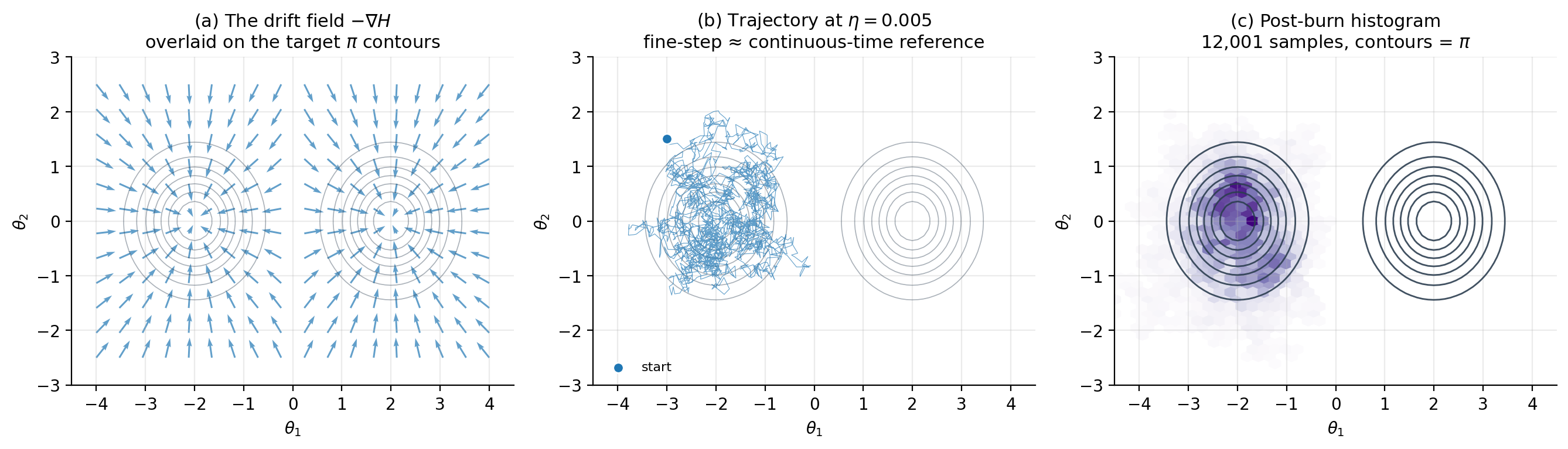
5. Overdamped Langevin dynamics

Theorem 2.1 admits an entire family of SDEs that target $\pi \propto e^{-H}$. The simplest member of the family — the one we get by setting $D = I$ and $Q = 0$ — is overdamped Langevin dynamics. This SDE is the continuous-time object that SGLD discretizes, so understanding it as a continuous process is the prerequisite for §6’s discrete-and-stochastic analysis.

5.1 The SDE

Take $D(\theta) = I$, the $d \times d$ identity, and $Q(\theta) \equiv 0$. The correction term $\Gamma$ vanishes (constant matrix entries have zero derivative), and Theorem 2.1’s drift collapses to $f(\theta) = -\nabla H(\theta)$. The complete-recipe SDE becomes

$$d\theta_t = -\nabla H(\theta_t)\, dt + \sqrt{2}\, dW_t, \qquad \qquad (5.1)$$

where $W_t$ is standard Brownian motion in $\mathbb{R}^d$. We will call (5.1) the overdamped Langevin SDE throughout. Some authors include a temperature parameter and write $\sqrt{2 k_B T}$ in front of $dW_t$ to emphasize the physics origin; we have absorbed $k_B T$ into the definition of $H$ so the noise prefactor is the bare $\sqrt{2}$. Section 5.4 says where the temperature went and why this is harmless.

5.2 Stationarity, free of charge

Substituting $D = I$, $Q = 0$ into Theorem 2.1 gives stationarity of $\pi \propto e^{-H}$ at no extra work. The probability current from §4 specializes to $J(\pi) = -\pi\, \nabla H + \nabla H \cdot \pi - \pi (\nabla \cdot I) = 0$, so detailed balance holds — the overdamped Langevin process is time-reversible. Among the SG-MCMC family, this is the most-symmetric case; SGHMC, RSGLD, and RMHMC all sacrifice reversibility to gain mixing speed.

The fact that we get stationarity from a one-line specialization of §4 is the payoff for setting up the complete-recipe machinery early. We will not redo the calculation each time we introduce a new method — we just check what $(D, Q)$ they correspond to and quote Theorem 2.1.

5.3 Geometric picture: gradient flow plus noise

To see what (5.1) does mechanically, decompose the right-hand side into its two pieces. The drift $-\nabla H(\theta)\, dt$ is the gradient flow of $H$ — it pulls the trajectory toward local minima of $H$, which are local maxima of $\pi$. Without the noise, $\theta_t$ would converge to the nearest mode of $\pi$ and stay there; this is exactly the maximum-a-posteriori (MAP) limit, which corresponds to the deterministic ODE $\dot \theta = -\nabla H$.

The noise $\sqrt{2}\, dW_t$ injects isotropic Brownian fluctuations of unit variance per unit time. The fluctuations prevent collapse to the mode and are precisely calibrated — through the $\sqrt{2}$ factor — to cancel the gradient pull and produce the stationary measure $\pi$. Concretely: a particle near the mode is buffeted away from it by the noise, then pulled back by the drift; on long time scales, the visit frequency to a region $A$ equals $\pi(A)$.

The isotropy of the noise is what creates the geometric trouble that motivates the rest of the topic. If $\pi$ is itself anisotropic — say a long thin Gaussian with one variance much larger than the other — the drift along the short direction is strong, while along the long direction the drift is weak; the noise, however, is the same magnitude in every direction. The result is fast equilibration of the short axis and slow random-walk diffusion along the long axis, with mixing time scaling as the square of the condition number of the curvature matrix at the mode (Roberts and Stramer 2002). Hierarchical models like Neal’s funnel make this pathology much worse, because the local condition number explodes near $v \to -\infty$. We will see the funnel break overdamped Langevin in §10 and fix the problem with a Riemann-manifold metric.

Re-running chain…

5.4 Why “overdamped”

The name has a physical origin worth keeping in mind. Newton’s equation for a particle of mass $m$ in a potential $U$ with friction coefficient $\gamma$ at temperature $T$ is

$$m \ddot \theta = -\nabla U(\theta) - \gamma \dot \theta + \sqrt{2 \gamma k_B T}\, \dot W_t,$$

a second-order SDE in $\theta$ (or a first-order SDE in the position–momentum pair). The overdamped limit takes $m \to 0$ — equivalently, friction dominating inertia — which makes the $\ddot \theta$ term negligible and leaves the first-order equation $\gamma \dot \theta = -\nabla U + \sqrt{2 \gamma k_B T}\, \dot W_t$. Dividing by $\gamma$, absorbing $k_B T / \gamma$ into the time scale, and identifying $H = U / (k_B T)$ recovers (5.1). The physics name is “overdamped” because friction dominates inertia; the practical consequence is that the dynamics has no momentum and so cannot ballistically traverse low-density valleys — every move is local. Section 7 brings momentum back by working with the underdamped Langevin SDE, which keeps mass and friction both finite. SGHMC is its discretization.

In MCMC vocabulary, “overdamped” is shorthand for “first-order, no-momentum” SDEs, and “underdamped” for “second-order, with-momentum” ones. The physics name matters because the Hamiltonian-vs-friction trade-off is exactly what controls mixing speed in §7.

6. Stochastic-Gradient Langevin Dynamics (SGLD)

§5 gave us the continuous-time Langevin SDE. SGLD is what we get when we apply two practical reductions in sequence: discretize the SDE with Euler–Maruyama (already developed in §3.4), and replace the full-data gradient with a mini-batch estimator (because for posteriors over deep-network weights with large $N$, the full-batch gradient is the dominant per-step cost). Welling and Teh (2011) showed that under a mild step-size schedule, both reductions wash out asymptotically and the chain still samples from $\pi$. This section formalizes that argument.

6.1 Euler–Maruyama on the overdamped Langevin SDE

Apply (3.3) to (5.1). The drift coefficient is $a(\theta) = -\nabla H(\theta)$ and the diffusion coefficient is the constant $\sqrt{2}\, I$, so the update reads

$$\theta_{n+1} = \theta_n - \eta\, \nabla H(\theta_n) + \sqrt{2\eta}\, \xi_n, \qquad \xi_n \overset{\text{iid}}{\sim} \mathcal{N}(0, I_d). \qquad \qquad (6.1)$$

This is what we’d run if we could compute the full-data gradient at every step. The $\sqrt{2\eta}$ noise scaling is critical — substitute $\eta$ for $\sqrt{2\eta}$ and the Euler–Maruyama scheme converges to the wrong SDE (one with a different stationary distribution). bayesian-neural-networks §6.2 wrote the same update with the alternative parametrization $\theta - (\eta'/2)\nabla U + \sqrt{\eta'}\, \xi$, equivalent to (6.1) under $\eta' = 2\eta$. Both forms appear in the literature; we use (6.1) throughout because the $\sqrt{2}$ pairs cleanly with Theorem 2.1’s $\sqrt{2D}$.

6.2 The mini-batch gradient estimator

For a Bayesian posterior with $N$ conditionally independent observations,

$$H(\theta) = -\log p(\theta) - \sum_{i=1}^N \log p(y_i \mid \theta), \qquad \nabla H(\theta) = -\nabla \log p(\theta) - \sum_{i=1}^N \nabla \log p(y_i \mid \theta).$$

The full gradient costs $O(N)$ per step; for $N = 10^6$ this is the bottleneck. Replace the data sum with a stochastic estimator built from a uniformly-sampled mini-batch $S \subset \{1, \ldots, N\}$ of size $B \ll N$:

$$\hat \nabla H_B(\theta) = -\nabla \log p(\theta) - \frac{N}{B} \sum_{i \in S} \nabla \log p(y_i \mid \theta). \qquad \qquad (6.2)$$

The estimator is unbiased: $\mathbb{E}_S[\hat \nabla H_B(\theta)] = \nabla H(\theta)$. Its variance scales with $1/B$ — concretely, $\mathrm{Var}_S[\hat \nabla H_B(\theta)] = \frac{N(N-B)}{B} \cdot \mathrm{Var}_{i \sim \text{unif}}[\nabla \log p(y_i \mid \theta)]$, where the inner variance is taken over a uniform draw from the dataset.

The SGLD update is now (6.1) with $\nabla H$ replaced by $\hat \nabla H_B$:

$$\theta_{n+1} = \theta_n - \eta_n\, \hat \nabla H_{B}(\theta_n) + \sqrt{2 \eta_n}\, \xi_n. \qquad \qquad (6.3)$$

Two sources of randomness now drive the chain: the deliberately-injected Brownian noise $\sqrt{2\eta_n}\, \xi_n$ scaling as $\sqrt{\eta_n}$, and the unwanted gradient noise $\eta_n \cdot (\hat \nabla H_B - \nabla H)$ scaling as $\eta_n$. The asymptotic-exactness argument hinges on which one dominates as $\eta_n \to 0$.

6.3 The Welling–Teh schedule and asymptotic exactness

Welling and Teh (2011) observed that as $\eta_n \to 0$, the gradient noise term shrinks faster than the injected noise ($\eta_n$ versus $\sqrt{\eta_n}$), so the gradient noise becomes asymptotically negligible. Run the chain with a step-size schedule satisfying

$$\sum_{n=1}^\infty \eta_n = \infty \quad \text{and} \quad \sum_{n=1}^\infty \eta_n^2 < \infty, \qquad \qquad (6.4)$$

and the time-averaged sample statistics converge to expectations under $\pi$ as $n \to \infty$. The first condition guarantees the chain travels arbitrarily far — without it, the chain stalls before it has explored. The second condition guarantees that the cumulative gradient-noise variance is finite — without it, the gradient noise dominates the injected noise and the chain becomes a stochastic-gradient-descent variant (which converges to the MAP, not to $\pi$). The standard polynomial schedule $\eta_n = a / (b + n)^\gamma$ with $\gamma \in (0.5, 1]$ satisfies both conditions.

What this does not require: a Metropolis–Hastings accept/reject step. Standard MCMC methods would correct the discretization error with an MH acceptance probability that involves the full-data likelihood, which would defeat the purpose of mini-batching. SGLD’s asymptotic exactness comes from the vanishing noise floor, not from MH rejection. The price is that we cannot stop at finite $\eta$ and expect to be sampling exactly from $\pi$; §8 quantifies the bias incurred when we do.

6.4 Constant step size: the BNN regime

In practice — including throughout BNN §6 — SGLD is run with a constant step size, not a decreasing schedule. The motivation is mixing speed: a constant $\eta$ keeps the chain moving briskly, whereas the Welling–Teh schedule slows the chain down arbitrarily as $n \to \infty$. The cost is that the chain’s stationary distribution is shifted from $\pi$ by an amount that scales as $O(\eta + B^{-1})$; this is the Vollmer–Zygalakis–Teh (2016) bound which we prove in §8. For most ML applications — large $N$, moderate-precision posterior estimates, and a budget that constrains $n$ to be much less than the polynomial-schedule’s mixing time — the constant-$\eta$ regime dominates the bias-variance trade-off. We use it throughout BNN’s worked examples and revisit the bias quantitatively in §8.

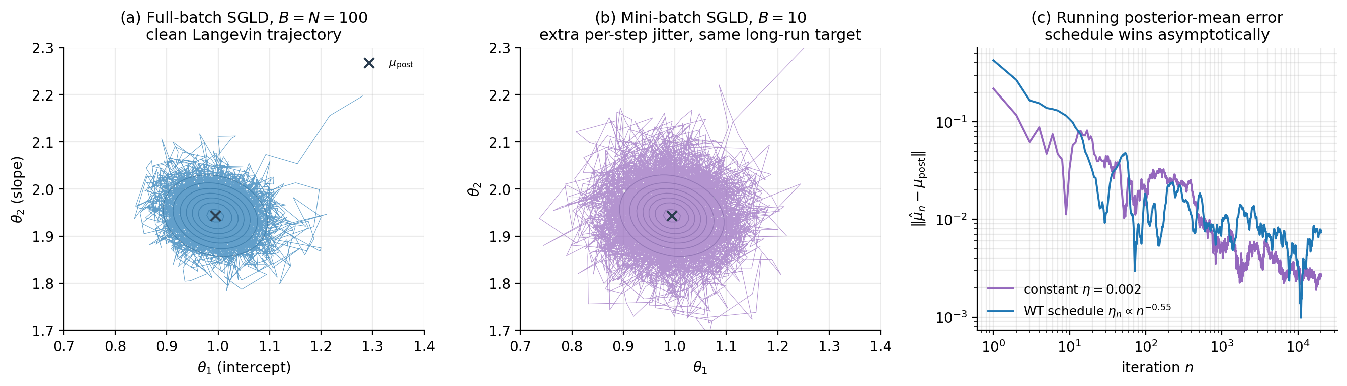
6.5 Algorithm and worked example

The vanilla SGLD algorithm with mini-batches is

input: gradient estimator ∇̂H_B, step size η (or schedule {η_n}),
       initial θ_0, batch size B, total iterations T, dataset size N
for n = 0, 1, ..., T - 1:
    sample S ⊂ {1, ..., N} uniformly without replacement, |S| = B
    g ← ∇̂H_B(θ_n; S)                              # using equation (6.2)
    sample ξ ~ N(0, I_d)
    θ_{n+1} ← θ_n - η_n · g + √(2 η_n) · ξ
return {θ_n : n = 1, ..., T}

The viz below runs SGLD on a 2D Bayesian linear regression with $N = 100$ synthetic observations, comparing the full-batch chain ($B = N$), a mini-batch chain ($B$ user-set), and a constant-$\eta$ chain against a Welling–Teh-schedule chain on the running posterior-mean error. The figure shows what the theory predicts: the full-batch and mini-batch chains have the same long-run distribution (panels (a) and (b) trace out the same Gaussian posterior, just with different per-step jitter), and the schedule chain’s running-mean error decays to zero while the constant-$\eta$ chain’s stalls at a positive bias floor (panel (c) — exactly the $O(\eta + B^{-1})$ behavior of §8).

Loading…

7. Underdamped Langevin and SGHMC

The overdamped dynamics in §§5–6 has no momentum: every step’s direction is determined by the local gradient, plus isotropic noise. On well-conditioned targets this is fine, but on anisotropic targets — including most posteriors over neural-network weights — it produces slow random-walk mixing along the long axes. The fix, due to Hamiltonian Monte Carlo (Duane et al. 1987; Neal 2011), is to extend the state space with a momentum variable and let the chain move ballistically along low-density valleys. In its stochastic-gradient form, this is SGHMC (Chen, Fox, and Guestrin 2014).

7.1 The underdamped Langevin SDE

Introduce a momentum variable $r \in \mathbb{R}^d$ with the same dimension as $\theta$, a positive-definite mass matrix $M$ (typically chosen as a multiple of the identity), and a positive-definite friction matrix $C$. The extended energy is the Hamiltonian

$$H(\theta, r) = U(\theta) + \tfrac{1}{2}\, r^\top M^{-1} r, \qquad \qquad (7.1)$$

where the first term is the original target energy ($U = -\log \pi$ up to constant) and the second term is the kinetic energy. The underdamped Langevin SDE on $(\theta, r) \in \mathbb{R}^{2d}$ is

$$\begin{aligned} d\theta_t &= M^{-1} r_t\, dt, \\ dr_t &= -\nabla U(\theta_t)\, dt - C M^{-1} r_t\, dt + \sqrt{2 C}\, dW_t. \end{aligned} \qquad \qquad (7.2)$$

The position equation is purely deterministic — only the momentum gets noise. The momentum equation has three parts: the Hamiltonian force $-\nabla U$ (rotation around level sets of $H$), the linear friction $-C M^{-1} r$ that bleeds energy out of the momentum subspace, and the calibrated noise $\sqrt{2C}\, dW$ that pumps energy back in. The friction–noise pairing is what keeps the joint distribution stationary; we verify this in §7.2.

7.2 Stationarity from Theorem 2.1

We take the Theorem-2.1 dispatch in (7.2) seriously: choose the joint state $(\theta, r)$ to live in $\mathbb{R}^{2d}$, and pick

$$D(\theta, r) = \begin{pmatrix} 0 & 0 \\ 0 & C \end{pmatrix}, \qquad Q(\theta, r) = \begin{pmatrix} 0 & -I \\ I & 0 \end{pmatrix}, \qquad \qquad (7.3)$$

both of size $2d \times 2d$ and treated as constants in $(\theta, r)$. The matrix $D$ is positive semi-definite (the position block is zero, but the momentum block is $C \succ 0$). The matrix $Q$ is skew-symmetric ($Q^\top = -Q$), which is the only nontrivial condition.

Compute Theorem 2.1’s drift. With $\nabla H = (\nabla U(\theta),\, M^{-1} r)^\top$,

$$(D + Q)\, \nabla H = \begin{pmatrix} 0 & -I \\ I & C \end{pmatrix} \begin{pmatrix} \nabla U \\ M^{-1} r \end{pmatrix} = \begin{pmatrix} -M^{-1} r \\ \nabla U + C M^{-1} r \end{pmatrix},$$

so the drift is $f = -(D+Q)\nabla H + \Gamma$ with $\Gamma = 0$ (constant matrices have zero $\Gamma$):

$$f = \begin{pmatrix} M^{-1} r \\ -\nabla U - C M^{-1} r \end{pmatrix}.$$

That matches (7.2) exactly. Theorem 2.1 then gives joint stationarity of

$$\pi(\theta, r) \propto \exp\!\bigl(-H(\theta, r)\bigr) = \underbrace{\exp(-U(\theta))}_{\propto\, \pi_\theta(\theta)} \cdot \underbrace{\exp\bigl(-\tfrac{1}{2} r^\top M^{-1} r\bigr)}_{\propto\, \mathcal{N}(0, M)},$$

so the target posterior $\pi_\theta$ and the Gaussian momentum prior $\mathcal{N}(0, M)$ are independent under the joint stationary measure.

Note that $Q \neq 0$, so $J(\pi) \neq 0$ pointwise — the dynamics is cyclically stationary, not detailed-balanced. Probability mass circulates around level sets of $H$ without accumulating, exactly as our §4.4 dichotomy predicted.

7.3 Marginalization recovers the target

Run (7.2) until equilibrium and project the trajectory onto the $\theta$-coordinate. Because $\pi(\theta, r) = \pi_\theta(\theta) \cdot \mathcal{N}(r; 0, M)$ factors, the marginal of the joint stationary on $\theta$ is exactly the target:

$$\int \pi(\theta, r)\, dr = \pi_\theta(\theta).$$

This is why we can ignore the momentum samples and report only the position samples as draws from the posterior. The momentum is auxiliary computational machinery; the posterior was always on $\theta$ alone.

7.4 Discretization

The simplest discretization of (7.2) is Euler–Maruyama applied to both equations simultaneously, giving

$$\begin{aligned} \theta_{n+1} &= \theta_n + \eta\, M^{-1} r_n, \\ r_{n+1} &= (I - \eta\, C M^{-1})\, r_n - \eta\, \nabla U(\theta_n) + \sqrt{2 \eta C}\, \xi_n, \end{aligned} \qquad \qquad (7.4)$$

with $\xi_n \sim \mathcal{N}(0, I_d)$. This is the form used in bayesian-neural-networks §7.2 — re-derived here as the discretization of (7.2) rather than as an isolated recipe. More accurate discretizations exist (Chen, Fox, and Guestrin 2014 give a friction-aware leapfrog, and Brooks et al. 2011 review symplectic alternatives), but (7.4) is what we use throughout because the additional accuracy is small at the $\eta$ values that make the §8 bias bound tight.

7.5 Mini-batches and the friction–noise calibration

Replace the full-data gradient $\nabla U(\theta)$ with the mini-batch estimator $\hat \nabla U_B(\theta)$ from (6.2). The momentum update becomes

$$r_{n+1} = (I - \eta C M^{-1})\, r_n - \eta\, \hat \nabla U_B(\theta_n) + \sqrt{2 \eta C}\, \xi_n.$$

The mini-batch gradient noise injects an extra covariance $\eta^2\, V(\theta_n)$ into the momentum, where $V(\theta) = \mathrm{Cov}_S[\hat \nabla U_B(\theta)]$ is the per-step gradient-estimator variance at $\theta$. Chen, Fox, and Guestrin (2014) observed that this extra variance can be partially absorbed into the calibrated noise by replacing $C$ with $C - \tfrac{\eta}{2} V(\theta)$ in the $\sqrt{2 \eta \cdot}\, \xi_n$ term. In practice — including throughout BNN §7 — $\eta$ is small enough that the correction is dropped: $V(\theta)$ is hard to estimate, $\eta \cdot V(\theta)$ is much smaller than $C$, and the resulting bias is the same $O(\eta + B^{-1})$ that Vollmer–Zygalakis–Teh quantify in §8 anyway. The vanilla update (7.4) with $\hat \nabla U_B$ in place of $\nabla U$ is what we run.

7.6 Why momentum mixes faster

The underdamped chain’s mixing advantage on anisotropic targets is the same one HMC enjoys over Metropolis–Hastings random walks. On a long thin Gaussian $\pi \propto \exp\!\bigl(-\tfrac{1}{2} \theta^\top \Sigma^{-1} \theta\bigr)$ with condition number $\kappa = \lambda_{\max}(\Sigma) / \lambda_{\min}(\Sigma)$, overdamped Langevin’s mixing time scales as $O(\kappa)$ while underdamped Langevin’s scales as $O(\sqrt{\kappa})$ (Cheng et al. 2018). The intuition: a particle with momentum carries velocity through low-density valleys, whereas an overdamped particle has to diffuse step-by-step. For neural-network posteriors with curvature spread over many orders of magnitude, the difference is operational — $\kappa = 10^4$ gives a $100\times$ mixing advantage to SGHMC over SGLD.

The friction matrix $C$ controls the regime. Small $C$ approaches Hamiltonian dynamics — fast ballistic motion but weak ergodicity (the chain can take a long time to forget initial conditions). Large $C$ approaches overdamped Langevin — strong ergodicity but slow mixing. The sweet spot is intermediate; a common rule of thumb is $C \approx \sqrt{M}$ entrywise, which equalizes the friction and oscillation timescales.

7.7 Algorithm and worked example

The vanilla SGHMC algorithm (matching BNN §7.2) is

input: gradient estimator ∇̂U_B, step size η, friction C, mass M,
       initial θ_0, batch size B, total iterations T, dataset size N
sample r_0 ~ N(0, M)
for n = 0, 1, ..., T - 1:
    sample S ⊂ {1, ..., N} uniformly, |S| = B
    g ← ∇̂U_B(θ_n; S)
    sample ξ ~ N(0, I_d)
    r_{n+1} ← (I - η · C M⁻¹) · r_n - η · g + √(2 η C) · ξ
    θ_{n+1} ← θ_n + η · M⁻¹ · r_{n+1}
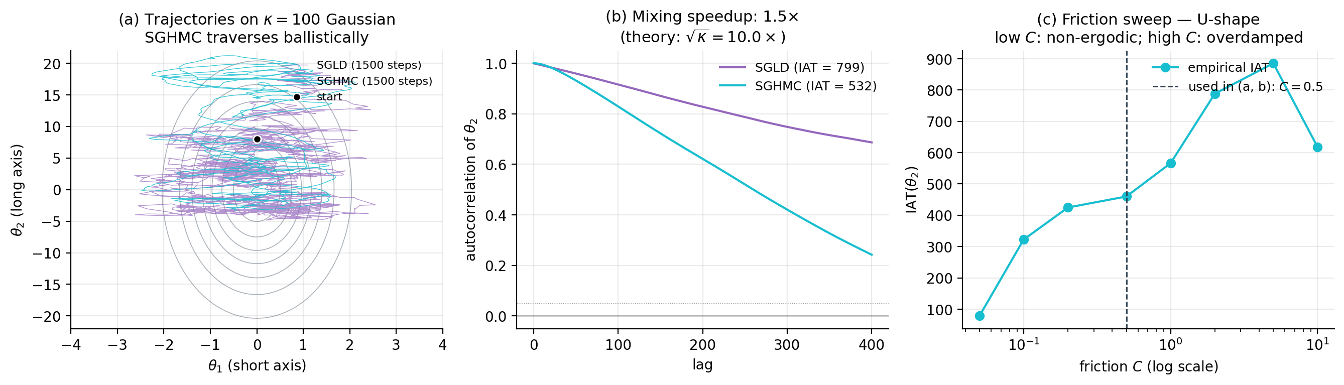
return {θ_n : n = 1, ..., T}

The viz below runs SGLD and SGHMC on a deliberately anisotropic 2D Gaussian (condition number $\kappa = 100$) and compares (a) trajectories, (b) per-coordinate autocorrelation functions, and (c) integrated autocorrelation time vs. friction $C$ for SGHMC. The figure makes the §7.6 scaling concrete: SGHMC’s IAT is smaller than SGLD’s at the optimal friction setting, and the $C$-dependence shows the predicted U-shape — too little friction makes the chain non-ergodic, too much makes it overdamped.

Loading…

8. Mini-batch finite-sample bias

§§5–7 set up the continuous-time SDEs and §6 quantified one source of error — the gradient-noise term that vanishes asymptotically under the Welling–Teh schedule. In practice we run constant-$\eta$ chains, often for far fewer iterations than the schedule would require for tight convergence. What does this cost us? The answer is given by Vollmer, Zygalakis, and Teh (2016): the bias of expectations under the chain’s stationary distribution is $O(\eta) + O(1/B)$, with explicit (though messy) constants. This section writes the decomposition out, states the bound, and answers the standing question of why we do not patch the bias with a Metropolis–Hastings accept/reject step.

8.1 Three sources of bias

Let $\hat \pi_n$ denote the law of $\theta_n$ under the SGLD chain (6.3) at step $n$, and $\pi$ the target posterior. There are three reasons $\hat \pi_n$ differs from $\pi$.

Discretization error. Even with the full-data gradient (no mini-batching), the Euler–Maruyama scheme is only weakly first-order accurate. The chain’s transition operator approximates $\exp(\eta \mathcal{L})$, where $\mathcal{L}$ is the generator of the SDE, with error $O(\eta^2)$ per step; over a finite time $T = n\eta$ this accumulates to $O(\eta)$ in expectations. Even at $B = N$ we are not sampling exactly from $\pi$; we are sampling from a perturbed measure that approaches $\pi$ as $\eta \to 0$.

Mini-batch gradient noise. Replacing $\nabla H$ with $\hat \nabla H_B$ injects an extra noise term into the chain. Concretely, the SGLD update with mini-batch gradient is

$$\theta_{n+1} = \theta_n - \eta \nabla H(\theta_n) + \bigl[-\eta\, \varepsilon_B(\theta_n) + \sqrt{2\eta}\, \xi_n\bigr],$$

where $\varepsilon_B(\theta) = \hat \nabla H_B(\theta) - \nabla H(\theta)$ is the mean-zero gradient-estimator error with covariance $V_B(\theta)$. The total per-step noise has covariance $2\eta\, I + \eta^2\, V_B(\theta_n)$. Compared to the full-batch case, the chain is effectively running with diffusion coefficient $I + \tfrac{\eta}{2} V_B$ instead of $I$ — the mini-batch noise inflates the diffusion in a state-dependent way, which biases the stationary distribution.

No Metropolis correction. Standard MCMC methods (Metropolis–Hastings, HMC) correct discretization error with an accept/reject step that ensures detailed balance with respect to $\pi$ at every iteration. SGLD and SGHMC drop this step. Why is the subject of §8.4; the consequence is that the chain has no built-in mechanism to remove the bias from the first two sources.

8.2 Decomposition argument

The cleanest way to see how the two error sources combine is to ask what SDE the SGLD chain is actually discretizing. Treating the mini-batch noise $\varepsilon_B(\theta)$ as Gaussian with covariance $V_B(\theta)$ — which is asymptotically correct as $B \to \infty$ by the central limit theorem — the per-step noise in (6.3) has covariance $2\eta\, I + \eta^2\, V_B(\theta_n)$. Pull a $2\eta$ out and write this as $2\eta \bigl[I + \tfrac{\eta}{2} V_B(\theta)\bigr]$. The chain is therefore (to leading order) the Euler–Maruyama discretization of the SDE

$$d\theta_t = -\nabla H(\theta_t)\, dt + \sqrt{2\bigl[I + \tfrac{\eta}{2} V_B(\theta_t)\bigr]}\, dW_t. \qquad \qquad (8.1)$$

The drift is unchanged from the original Langevin SDE (5.1), but the diffusion has acquired an extra state-dependent piece $\tfrac{\eta}{2} V_B(\theta)$. By Theorem 2.1 with $D(\theta) = I + \tfrac{\eta}{2} V_B(\theta)$ and $Q = 0$, this perturbed SDE has stationary distribution shifted from $\pi$. The shift is the second source of bias above.

For an unbiased mini-batch estimator with the $N/B$ rescaling of (6.2), the gradient covariance scales as $V_B(\theta) \asymp N^2 / B$ — so the bias contribution to expectations is $O(\eta \cdot V_B / N^2) = O(\eta / B)$ once we normalize back to per-datapoint units. Combining with the $O(\eta)$ discretization error from §8.1 gives the headline bound.

8.3 The Vollmer–Zygalakis–Teh theorem

The argument above is heuristic — it ignores the Euler–Maruyama discretization error, the corrections from the chain not being exactly at stationarity, and the dependence of constants on the test statistic $\phi$. Vollmer, Zygalakis, and Teh (2016) carried out the rigorous calculation using the generator of the SDE and the Poisson equation $\mathcal{L}\psi = \phi - \pi(\phi)$. Their main result, restated for our setting:

The proof is in §3 of VZT 2016 and uses Stein’s method via the Poisson equation; we do not reproduce it here. The takeaway is that (8.2) makes the §8.2 heuristic precise, with the constants $C_1, C_2$ depending on the smoothness of $H$ and $\phi$ and on the spectral gap of the generator $\mathcal{L}$. For our purposes, what matters is the form of the bound: bias decays linearly in $\eta$ at fixed $B$, and inversely in $B$ at fixed $\eta$.

8.4 Why we don’t add a Metropolis correction

A standard MCMC instinct, on seeing equation (8.2), is to add an MH accept/reject step to remove the bias. The acceptance probability for moving from $\theta_n$ to a proposal $\theta'$ would be

$$\alpha(\theta_n \to \theta') = \min\!\left\{1,\, \frac{\pi(\theta') q(\theta_n \mid \theta')}{\pi(\theta_n) q(\theta' \mid \theta_n)}\right\},$$

which requires evaluating $\pi(\theta) \propto \exp(-H(\theta)) = \exp\!\bigl(-\sum_i \log p(y_i \mid \theta) + \cdots\bigr)$ exactly. Computing $H$ requires summing log-likelihoods over all $N$ datapoints — exactly the $O(N)$ operation that mini-batching was introduced to avoid. An MH step at every iteration defeats the purpose.

There has been work on stochastic acceptance steps (Bardenet, Doucet, and Holmes 2014, 2017 — sub-sampling MH; Korattikara, Chen, and Welling 2014 — austerity MH), but the practical regimes in which these methods improve over plain SGLD are narrow. The accepted trade is to live with the $O(\eta + 1/B)$ bias and run with $\eta$ and $B$ chosen to keep that bias smaller than the Monte Carlo variance from finite $n$, which is $O(1/\sqrt{n})$ by ergodicity. For typical posterior-mean estimation in deep learning, $B = 32$ to $128$ and $\eta = 10^{-4}$ to $10^{-3}$ leave $O(\eta + 1/B) \approx 10^{-2}$, which is well below the Monte Carlo error from any practical chain length. The bias is real but operationally small.

8.5 Empirical verification

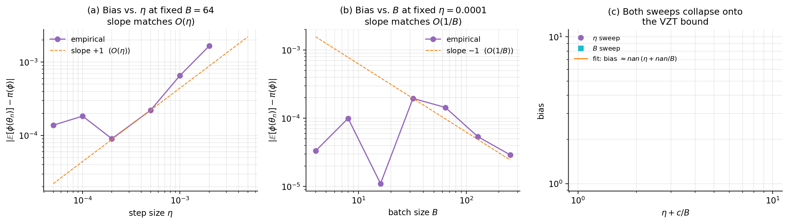
The viz below runs SGLD on the §6 Bayesian linear regression posterior with synthetic Gaussian gradient-estimator noise of covariance $\sigma_g^2 / B \cdot I$, allowing a clean sweep over both $\eta$ and $B$ independently. The figure shows the predicted scaling: panel (a) plots empirical bias against $\eta$ at fixed $B = 64$, panel (b) plots empirical bias against $B$ at fixed $\eta = 10^{-4}$, and panel (c) collapses both onto a single line by plotting bias against $\eta + c/B$ for the empirically-fit constant $c$. The slopes match the $O(\eta) + O(1/B)$ bound’s predictions: $+1$ in $\eta$, $-1$ in $B$.

Loading…

9. Bias-reduction strategies

Theorem 8.1 says SGLD’s bias is $O(\eta) + O(1/B)$. Both terms can be attacked. The discretization term $O(\eta)$ shrinks if we can afford a smaller $\eta$ (paying in mixing time) or schedule $\eta_n \to 0$ (paying in asymptotic chain length). The mini-batch term $O(1/B)$ shrinks if we can afford a larger batch (paying in per-step cost) or — more interestingly — if we can reduce the gradient-estimator variance $V_B(\theta)$ at fixed $B$ through control-variate techniques. This section catalogs the four standard moves: step-size annealing, stochastic-gradient control variates (SVRG-LD), zero-variance control variates (ZV-SGLD), and exact-subsampling MCMC.

9.1 The bias-reduction landscape

Each method trades a different resource for bias reduction. Step-size annealing pays in chain length: the Welling–Teh schedule (§6.3) eliminates the $O(\eta)$ term as $n \to \infty$, but the chain mixes ever more slowly along the way. Larger batches pay in per-step cost: doubling $B$ halves the $O(1/B)$ contribution but doubles the gradient-evaluation cost. Stochastic-gradient control variates pay in implementation complexity and a moderate amount of compute: SVRG-LD reduces $V_B(\theta)$ by an order of magnitude near the posterior mode, and ZV-SGLD leaves $V_B$ alone but reduces the variance of the estimator we ultimately care about. Exact-subsampling MCMC pays in algorithmic delicacy and the requirement that the likelihood is bounded or geometrically Lipschitz: it eliminates bias entirely while preserving the per-step subsampling speedup. The choice depends on what is cheap in the application.

9.2 Stochastic-gradient control variates: SVRG-LD

SVRG-LD (Dubey et al. 2016) borrows the variance-reduced gradient idea from SVRG (Johnson and Zhang 2013) and applies it inside SGLD. Pick a reference point $\tilde\theta$ at which the full-data gradient $\tilde g = \nabla U(\tilde\theta)$ has been computed, and rewrite the mini-batch gradient at the current $\theta_n$ as

$$\hat \nabla U_B^{\,\text{SVRG}}(\theta_n) = \tilde g + \frac{N}{B} \sum_{i \in S} \bigl[\nabla \log p(y_i \mid \theta_n) - \nabla \log p(y_i \mid \tilde\theta)\bigr]. \qquad \qquad (9.1)$$

The estimator is unbiased — the bracketed difference has mean zero by linearity of the data-sum — and the variance is bounded by

$$\mathrm{Var}\!\bigl[\hat \nabla U_B^{\,\text{SVRG}}(\theta_n)\bigr] \leq \frac{L^2 N^2}{B}\, \|\theta_n - \tilde\theta\|^2,$$

where $L$ is the Lipschitz constant of the per-data-point gradient $\nabla \log p(y_i \mid \cdot)$. The variance scales with the squared distance from the reference point, so when the chain is mixing in a small neighborhood of the mode and $\tilde\theta$ is updated periodically to track it, $V_B$ near the mode becomes orders of magnitude smaller than vanilla mini-batch. The amortized cost is $O(N/k + B)$ per step, where $k$ is the inner-loop length between reference updates; in practice $k = 50$–$200$ gives a 5–20× variance reduction at modest extra cost.

The trade is geometric: the variance bound is meaningful only when $\tilde\theta$ tracks $\theta_n$ closely, which means SVRG-LD shines on unimodal (or weakly multimodal) targets where the chain stays in one basin. On posteriors with widely-separated modes, $\|\theta_n - \tilde\theta\|$ stays large and the variance reduction degrades.

9.3 Zero-variance control variates: ZV-SGLD

A different attack on the same problem: instead of shrinking the gradient noise $V_B$, shrink the variance of the final estimator we care about. For an observable $\phi(\theta)$ whose posterior expectation we want, define the modified estimator

$$\hat \phi_{\text{ZV}}(\theta) = \phi(\theta) + \alpha^\top \nabla U(\theta), \qquad \qquad (9.2)$$

where $\alpha \in \mathbb{R}^d$ is a coefficient vector (which we will fit). Two facts about (9.2). First, the modification is unbiased under $\pi$:

$$\mathbb{E}_\pi\!\bigl[\alpha^\top \nabla U(\theta)\bigr] = \alpha^\top \int \pi(\theta)\, \nabla U(\theta)\, d\theta = -\alpha^\top \int \nabla \pi(\theta)\, d\theta = 0,$$

where the second equality uses $\nabla \pi = -\pi\, \nabla U$ and the third uses the divergence theorem on $\pi$. So $\mathbb{E}_\pi[\hat \phi_{\text{ZV}}] = \mathbb{E}_\pi[\phi]$. Second, the optimal $\alpha^*$ that minimizes $\mathrm{Var}_\pi[\hat \phi_{\text{ZV}}]$ has closed form:

$$\alpha^* = -\bigl[\mathrm{Cov}_\pi(\nabla U, \nabla U)\bigr]^{-1} \mathrm{Cov}_\pi(\nabla U, \phi),$$

which can be estimated empirically from the SGLD chain itself. Mira, Solgi, and Imparato (2013) showed that for exact MCMC samples, ZV control variates can reduce estimator variance by 100× or more; for SGLD chains, the reduction is more modest (typically 5–20×) because the estimator inherits both the chain’s residual bias and noise in the $\hat\alpha$ estimate.

The strength of ZV-SGLD is that $\nabla U(\theta)$ is already computed at every chain step (it’s the SGLD gradient), so the control variate is essentially free. The weakness is that the linear control variate (9.2) only kills the part of $\phi$‘s variation that is correlated with $\nabla U$; nonlinear control variates of the form $\hat\phi = \phi + \alpha^\top \nabla U + \beta^\top \nabla^2 U \mathbf{1}$ (or higher polynomials) help on non-Gaussian posteriors but are more expensive to fit.

9.4 Step-size annealing

Already presented in §6.3 as the Welling–Teh schedule. From the bias perspective, annealing eliminates the $O(\eta)$ term asymptotically by sending $\eta_n \to 0$. The schedule $\eta_n = a / (b + n)^\gamma$ with $\gamma \in (0.5, 1]$ is the standard choice. The cost is mixing-time inflation: the integrated autocorrelation time grows as $\eta_n^{-1}$ for small $\eta_n$, so the chain wanders ever more slowly. In practice, annealing is used as a finishing phase — run constant-$\eta$ SGLD until the chain reaches stationarity, then switch to the schedule for the final precision-pinning iterations.

9.5 Exact-subsampling MCMC

The most ambitious bias-reduction strategy gives up the constant-$\eta$ approximation entirely and aims for unbiased samples from $\pi$ while still subsampling the data. Two methods are now standard.

Subsampling Metropolis–Hastings (Bardenet, Doucet, and Holmes 2014, 2017). Replace the full log-likelihood ratio in the MH acceptance probability with a stochastic estimate from a sub-sample. The sub-sample size grows adaptively: when the proposed move is “obviously” accepted or rejected (the estimated log-ratio is far from zero), a small batch suffices; when the proposal is borderline, more data are evaluated until the answer is statistically reliable. The chain’s stationary distribution is exactly $\pi$, with average per-step cost $O(\sqrt N)$ under regularity assumptions (Lipschitz log-likelihoods, Gaussian-like proposal distributions). The catch: the worst-case cost can degrade to $O(N)$, and the regularity assumptions exclude common cases such as latent-variable models with discrete components.

Firefly Monte Carlo (Maclaurin and Adams 2014). Augment the state space with binary indicator variables $z_i \in \{0, 1\}$ for each observation, where $z_i = 1$ marks the $i$-th data point as “active.” The chain alternates between $\theta$-updates (using only the active subset) and $z_i$-updates (which require evaluating $\log p(y_i \mid \theta)$ but only sample-by-sample). Properly designed, the marginal of the joint $(\theta, z)$ stationary distribution on $\theta$ is exactly $\pi$. Active-set sizes can be as low as $O(\sqrt N)$ when the likelihood factorizes well; the cost of $z$-updates is $O(N)$ per outer iteration but spread thinly.

For deep-learning-scale problems, neither method has displaced SGLD/SGHMC as the practical workhorse — the constants in their per-step costs and the geometric assumptions limit applicability. They remain the right tool when bias-free posterior samples are non-negotiable (e.g., regulatory or scientific reporting) and the dataset is large but not deep-learning-large.

9.6 Verdict

For typical Bayesian deep-learning posteriors at $N \in [10^4, 10^7]$, the cost-effectiveness ranking is approximately:

1. Vanilla SGLD/SGHMC  (baseline; bias O(η + 1/B))
2. + ZV-SGLD            (free; 5-20× estimator variance reduction)
3. + SVRG-LD            (modest cost; 5-20× gradient variance reduction)
4. + step-size schedule (asymptotic exactness; pays in mixing)
5. Subsampling MH       (exact; 10-100× cost over (1))
6. Firefly MC           (exact; 10-100× cost over (1))

The viz below runs vanilla SGLD, SVRG-LD, and ZV-SGLD on the §6 BLR posterior and compares (a) running estimates of $\mathbb{E}_\pi[\theta_1]$ and (b) the per-chain estimator standard error vs iteration count. ZV-SGLD typically wins by a factor of $\sim 10\times$ at zero compute overhead; SVRG-LD wins by a factor of $\sim 5\times$ at $\sim 30\%$ extra compute.

Re-running chains…

10. Riemann-manifold preconditioning

Vanilla SGLD and SGHMC use the Euclidean metric on parameter space — the noise injected at each step has covariance $I$ (or, for SGHMC, $C$ in the momentum subspace). When the target’s curvature is highly state-dependent, this calibration is mismatched: a step size that works at one location of the chain is wrong by orders of magnitude at another. The fix is to give parameter space a state-dependent Riemannian metric $G(\theta)$ that compensates for the local curvature, then run an SG-MCMC chain on the resulting manifold. Patterson and Teh (2013) introduced the Langevin version (RSGLD); Girolami and Calderhead (2011) had earlier introduced the Hamiltonian version (RMHMC) for full-batch HMC; Ma, Chen, and Fox (2015) unified both inside the complete-recipe framework. This section develops the Langevin case in detail and gestures at the Hamiltonian case.

10.1 The geometric pathology: Neal’s funnel

The motivating bad case is a posterior we have already seen — Neal’s funnel, the running example of probabilistic-programming §5. Take $v \sim \mathcal{N}(0, \sigma_v^2)$ and $x \mid v \sim \mathcal{N}(0, e^v)$, giving joint energy

$$H(v, x) = \frac{v^2}{2\sigma_v^2} + \frac{v}{2} + \frac{x^2}{2 e^v}.$$

The Hessian is

$$\nabla^2 H(v, x) = \begin{pmatrix} \sigma_v^{-2} + \tfrac{1}{2} x^2 e^{-v} & -x e^{-v} \\ -x e^{-v} & e^{-v} \end{pmatrix},$$

so the curvature in the $x$-direction is $e^{-v}$ — exponential in $v$. At $v = -5$ the curvature is $\sim 150$, and the local conditional density on $x$ is tightly concentrated ($\sigma \approx 0.08$); at $v = +5$ the curvature is $\sim 0.007$ and the local density is broad ($\sigma \approx 12$). A single step size cannot serve both regimes.

Vanilla SGLD on the funnel has update $\theta_{n+1} = \theta_n - \eta \nabla H + \sqrt{2\eta}\, \xi$. To make any progress in $x$ at $v = -5$, we need $\sqrt{2\eta} \cdot \xi_x$ to be at most $\sigma \approx 0.08$, which requires $\eta \lesssim 3 \cdot 10^{-3}$. With $\eta$ this small, the step in $v$ is at most $\sqrt{2\eta} \approx 0.08$ per iteration — meaningful $v$-mixing requires hundreds of thousands of steps. Probabilistic-programming’s fix was to reparametrize (introduce $\tilde x = x e^{-v/2}$ so that $\tilde x \sim \mathcal{N}(0, 1)$ unconditionally on $v$); SG-MCMC’s fix here is dual to that — keep the parametrization and change the metric.

10.2 The Riemannian-manifold framework

A Riemannian metric on $\mathbb{R}^d$ is a smooth map $G : \mathbb{R}^d \to \mathbb{R}^{d \times d}$ assigning a positive-definite matrix $G(\theta)$ at each point. Geometrically, $G(\theta)$ rescales distances locally — the inner product of two tangent vectors $u, w \in T_\theta \mathbb{R}^d$ is $\langle u, w \rangle_G = u^\top G(\theta) w$, and the corresponding gradient of $H$ is $G^{-1}(\theta) \nabla H(\theta)$ (the natural gradient). For our purposes the right intuition is that $G(\theta)^{-1}$ tells the chain how to scale its noise and gradient steps to match the local geometry.

The information metric is the canonical choice: $G(\theta)$ equals the local Hessian of $-\log \pi$ at $\theta$ (or its expectation, the Fisher information). Setting $G$ to the Hessian gives a chain whose effective step size is curvature-adapted everywhere — large where the target is broad, small where the target is narrow. Other diagonal approximations (RMSprop, Adam-style metrics) trade theoretical sharpness for cheaper updates; we cover one such approximation in §10.6.

10.3 RSGLD: the Langevin variant

Drop $G(\theta)^{-1}$ into Theorem 2.1’s diffusion coefficient: take

$$D(\theta) = G(\theta)^{-1}, \qquad Q(\theta) = 0.$$

The matrix $D$ is positive-definite, and $Q = 0$ trivially satisfies skew-symmetry. The correction $\Gamma_i(\theta) = \sum_j \partial_j (G^{-1})_{ij}$ is not zero — the entries of $G^{-1}$ depend on $\theta$ — and Theorem 2.1’s drift becomes

$$f(\theta) = -G(\theta)^{-1} \nabla H(\theta) + \nabla \!\cdot\! G^{-1}(\theta), \qquad \qquad (10.1)$$

where $(\nabla \cdot G^{-1})_i = \sum_j \partial_j (G^{-1})_{ij}$ is the matrix divergence of $G^{-1}$. The Riemann-manifold Langevin SDE is therefore

$$d\theta_t = \bigl[-G^{-1}(\theta_t)\, \nabla H(\theta_t) + \nabla \!\cdot\! G^{-1}(\theta_t)\bigr] dt + \sqrt{2 G^{-1}(\theta_t)}\, dW_t. \qquad \qquad (10.2)$$

By Theorem 2.1, the stationary distribution is $\pi \propto e^{-H}$ — exactly the target.

Discretizing with Euler–Maruyama gives the RSGLD update (Patterson and Teh 2013):

$$\theta_{n+1} = \theta_n + \eta\!\left[-G^{-1}(\theta_n) \hat \nabla H_B(\theta_n) + \nabla \!\cdot\! G^{-1}(\theta_n)\right] + \sqrt{2\eta}\, L(\theta_n) \xi_n, \qquad \qquad (10.3)$$

where $L(\theta_n)$ is any matrix square root (Cholesky factor) of $G^{-1}(\theta_n)$ and $\xi_n \sim \mathcal{N}(0, I_d)$. The structural difference from vanilla SGLD is the preconditioner $G^{-1}$ multiplying both the drift and the noise, and the new $\nabla \!\cdot\! G^{-1}$ term — the price we pay for state-dependent diffusion.

10.4 The correction term

The correction $\nabla \!\cdot\! G^{-1}(\theta)$ matters arithmetically and conceptually. Arithmetically, dropping it would make Theorem 2.1’s stationarity claim fail — the chain would target a different distribution, generally not $\pi$. Conceptually, the correction encodes the geometric requirement that the noise, when the metric is curved, has a built-in tendency to drift in the direction of decreasing volume; the $\nabla \!\cdot\! G^{-1}$ term cancels that tendency.

For diagonal metrics $G^{-1}(\theta) = \mathrm{diag}(g_1(\theta), \ldots, g_d(\theta))$, the correction simplifies to $(\nabla \!\cdot\! G^{-1})_i = \partial_i g_i(\theta)$. For the funnel-adapted metric we use in §10.6, $G^{-1}(v, x) = \mathrm{diag}(1, e^v)$ — depending on $v$ but not on $x$, and only in the second coordinate. The correction $(\nabla \!\cdot\! G^{-1})_v = \partial_v \cdot 1 = 0$ and $(\nabla \!\cdot\! G^{-1})_x = \partial_x e^v = 0$, so it vanishes identically. The funnel demo therefore needs no correction term, which lets us isolate the preconditioner’s effect cleanly. For the Fisher metric (full Hessian of $H$), the correction is generically nonzero and must be computed.

10.5 RMHMC and the underdamped extension

The Hamiltonian counterpart of RSGLD generalizes (7.2) by replacing the Euclidean kinetic energy $\tfrac{1}{2} r^\top M^{-1} r$ with a state-dependent kinetic energy $\tfrac{1}{2} r^\top G^{-1}(\theta) r$. The modified Hamiltonian is

$$H_R(\theta, r) = U(\theta) + \tfrac{1}{2} r^\top G^{-1}(\theta) r + \tfrac{1}{2} \log \det G(\theta),$$

where the $\log \det$ term is the volume correction needed to make the joint $\pi(\theta, r) \propto \exp(-H_R)$ have the correct $\theta$-marginal. The corresponding $D, Q$ choice in Theorem 2.1 generalizes (7.3) to use $G^{-1}$-blocks; details are in Ma, Chen, and Fox (2015) and Girolami and Calderhead (2011). Discretizing Riemann-manifold Hamiltonian dynamics is more involved than RSGLD because the kinetic energy depends on $\theta$ through $G$; a generalized leapfrog scheme (Girolami and Calderhead 2011 §3.3) is the standard choice.

10.6 Worked example: the funnel with and without preconditioning

The viz below implements RSGLD on the funnel with metric $G(v, x) = \mathrm{diag}(1, e^{-v})$, hence $G^{-1}(v, x) = \mathrm{diag}(1, e^v)$. The chain’s effective dynamics, after substituting (10.3), become

$$\begin{aligned} v_{n+1} &= v_n - \eta \cdot \partial_v H + \sqrt{2\eta}\, \xi_v, \\ x_{n+1} &= x_n - \eta \cdot e^{v_n} \partial_x H + \sqrt{2\eta\, e^{v_n}}\, \xi_x. \end{aligned}$$

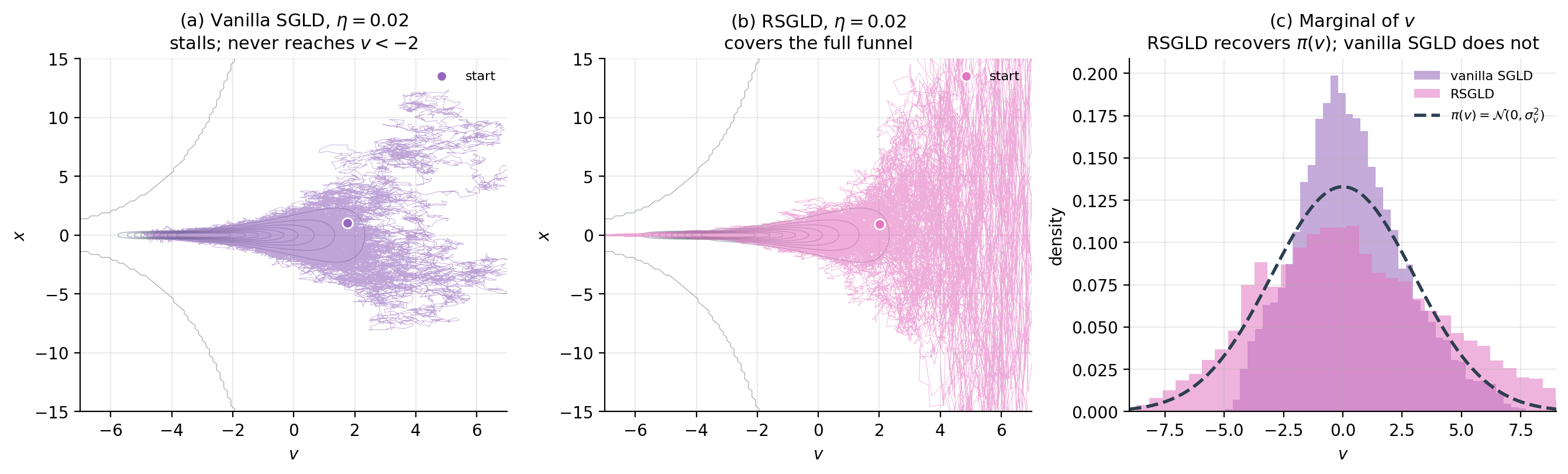
The $v$-update is unchanged from vanilla SGLD. The $x$-update simplifies dramatically: $\partial_x H = x e^{-v}$, so $-e^v \partial_x H = -x$, recovering an Ornstein–Uhlenbeck process on $x$ with unit drift coefficient. The state-dependent curvature has been absorbed into the metric. The figure shows the dramatic mixing improvement: vanilla SGLD spends most of its time in the wide neck of the funnel and never explores the narrow throat below $v < -2$, whereas RSGLD covers the full funnel uniformly and recovers the marginal $\mathcal{N}(0, \sigma_v^2)$ for $v$.

Loading…

11. Computational Notes

The math in §§3–10 establishes that SGLD, SGHMC, and RSGLD are correct. The implementation in production requires more care than the toy chains we ran on 2D targets — neural-network parameters live in dictionaries-of-tensors, gradients come from autodiff frameworks, and the difference between a working chain and a silently broken one often comes down to tensor-shape arithmetic. This section ships the canonical implementation patterns alongside the diagnostic helpers needed to verify a chain has reached stationarity.

11.1 Vanilla SGLD step (PyTorch, parameter-iterating)

The cleanest production-ready SGLD implementation iterates over model.parameters(), computing the gradient via autodiff and updating each parameter tensor in place. The key API decisions are: (a) the noise scale $\sqrt{2\eta}$ pairs with the loss-as-negative-log-posterior convention, where the prior contribution must be added explicitly to the loss as additive regularization; (b) the mini-batch gradient is naturally produced by PyTorch dataloaders, so no manual subsampling is required; (c) the torch.no_grad() context is essential — the parameter update must not be tracked as a differentiable operation.

def sgld_step(model, loss, eta, prior_lambda, generator=None):
    """One SGLD iteration on a torch.nn.Module.

    Args:
        model: torch.nn.Module whose .parameters() will be updated in place.
        loss: scalar Tensor — the negative log-likelihood for the current
              mini-batch, summed and rescaled by N/B if working with the mean.
        eta: step size η.
        prior_lambda: λ such that prior contribution ½λ‖w‖² is added to U.
        generator: torch.Generator for reproducibility (optional).
    """
    model.zero_grad()
    loss.backward()
    with torch.no_grad():
        for p in model.parameters():
            if p.grad is None:
                continue
            grad = p.grad + prior_lambda * p
            noise = torch.randn(p.shape, generator=generator, device=p.device, dtype=p.dtype)
            p.add_(-eta * grad + math.sqrt(2 * eta) * noise)

This matches BNN §6.5’s worked-example function up to the explicit prior-gradient handling; we pulled the prior out of the loss so the function works with any user-supplied likelihood term.

11.2 SGHMC step with optional preconditioning

SGHMC requires per-parameter momentum buffers, which we attach to the module as a side-channel dictionary keyed by parameter name. The friction coefficient $C$ and mass $M$ default to scalars (uniform across parameters) but can be passed as per-tensor dictionaries for layer-specific tuning.

def sghmc_step(model, loss, eta, C, M, momentum_buffers, prior_lambda, generator=None):
    """One SGHMC iteration. momentum_buffers is a dict {name: Tensor} holding
    per-parameter momentum r; must be initialized externally before the first
    call. Updates both model.parameters() and momentum_buffers in place."""
    model.zero_grad()
    loss.backward()
    with torch.no_grad():
        for name, p in model.named_parameters():
            if p.grad is None:
                continue
            r = momentum_buffers[name]
            grad = p.grad + prior_lambda * p
            xi = torch.randn(p.shape, generator=generator, device=p.device, dtype=p.dtype)
            r.mul_(1 - eta * C / M).add_(-eta * grad + math.sqrt(2 * eta * C) * xi)
            p.add_(eta * r / M)

Two operational notes. First, the momentum buffer initialization should match the kinetic-energy stationary distribution: r0 = sqrt(M) * randn(...). Initializing at zero introduces a transient that takes $O(1/(\eta C))$ iterations to wash out. Second, prior_lambda here applies only to the gradient (entering the momentum update); the prior does not directly modify the position update.

11.3 RSGLD step with diagonal-metric callback

RSGLD admits a simpler implementation when the metric is diagonal — the matrix square root is element-wise, and the divergence $\nabla \!\cdot\! G^{-1}$ has the simple form $(\partial_i g_i^{-1})$. We expose the metric and its divergence as callbacks so the same step function works for any diagonal preconditioner.

def rsgld_step_diagonal(theta, grad_U_fn, G_inv_diag_fn, div_G_inv_fn, eta, rng):
    """One RSGLD step with a diagonal Riemannian metric. Returns the updated θ."""
    G_inv = G_inv_diag_fn(theta)
    correction = div_G_inv_fn(theta)
    g = grad_U_fn(theta)
    drift = -G_inv * g + correction
    noise = np.sqrt(2 * eta) * np.sqrt(G_inv) * rng.standard_normal(theta.shape)
    return theta + eta * drift + noise

Sanity check: when G_inv_diag_fn returns np.ones(d) and div_G_inv_fn returns zeros, this reduces to vanilla SGLD. For the §10.6 funnel metric, G_inv_diag_fn(theta) = np.array([1.0, np.exp(theta[0])]) and div_G_inv_fn returns zeros (verified in §10.4).

11.4 ESS, IAT, and R̂ diagnostics

The diagnostic utilities autocorr, integrated_autocorr_time, effective_sample_size cover the single-chain case. For multi-chain SG-MCMC runs, the standard diagnostic is Gelman–Rubin’s $\hat R$, which compares within-chain to between-chain variance and signals lack of convergence when $\hat R > 1.01$.

def gelman_rubin_rhat(chains):
    """R̂ statistic over multiple chains. Convergence requires R̂ < 1.01."""
    chains = np.asarray(chains, dtype=float)
    if chains.ndim == 2:
        chains = chains[..., None]
    n_chains, n_iter, d = chains.shape
    chain_means = chains.mean(axis=1)
    chain_vars = chains.var(axis=1, ddof=1)
    grand_mean = chain_means.mean(axis=0)
    B = n_iter * ((chain_means - grand_mean) ** 2).sum(axis=0) / max(n_chains - 1, 1)
    W = chain_vars.mean(axis=0)
    var_hat = (n_iter - 1) / n_iter * W + B / n_iter
    return np.sqrt(var_hat / W).squeeze()

For SG-MCMC chains, $\hat R$ is necessary but not sufficient — the chains may agree with each other while all sampling from a slightly biased distribution (the §8 finite-sample bias). The standard practice is to combine $\hat R < 1.01$ with a separate check on either the §8 bias-vs-$\eta$ scaling or a comparison to a reference chain (NUTS at moderate $N$).

11.5 Hyperparameter recipes

The largest gap between SG-MCMC theory and SG-MCMC practice is hyperparameter selection. The following defaults work for the regimes we have studied; they are starting points, not optimal values.

Regime	$\eta$	$B$	$C$ (SGHMC)	Reference
Bayesian logistic regression, $N \sim 10^3$	$10^{-3}$	32	0.1	this notebook §6, §12
Bayesian neural network, MNIST-scale	$10^{-5}$	128	0.05	BNN §§6, 7
Bayesian neural network, ImageNet-scale	$10^{-6}$	512	0.01	Wenzel et al. 2020
Hierarchical model with funnel pathology	$10^{-2}$ (RSGLD)	64	—	§10.6

A useful rule-of-thumb: pick $\eta$ so that the per-step parameter change $\eta \|\nabla U\|$ is $\sim 10\%$ of the standard deviation of the chain at stationarity. This balances the discretization error against the noise floor.

12. SG-MCMC in Machine Learning

We have spent eleven sections developing the SG-MCMC framework on toy 2D targets. The point of doing so was always to deploy the methods on real ML problems — neural-network posteriors over hundreds of thousands of parameters, Bayesian logistic regressions over millions of observations, hierarchical models with badly-conditioned geometry. This closing section is the practical pay-off: a head-to-head with NUTS on a controlled benchmark, the regime where SG-MCMC genuinely wins, and a decision tree that says when to reach for which method.

12.1 The head-to-head benchmark

The natural way to compare SG-MCMC and NUTS is effective sample size per second of wall-clock time (ESS/sec). NUTS produces high-quality samples but pays a per-step cost of $O(N \cdot \text{tree depth})$ with full-data gradients; SG-MCMC produces lower-quality (biased) samples at $O(B)$ per step with mini-batched gradients. The crossover happens where NUTS’s per-step cost outweighs its sampling-quality advantage.

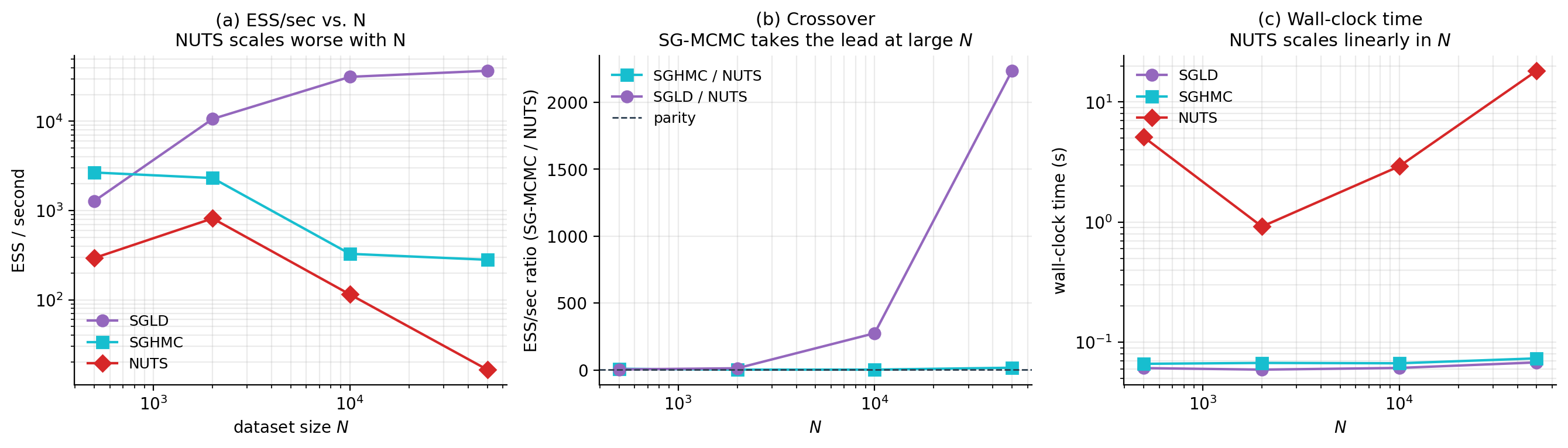
Our benchmark target is Bayesian logistic regression with $D = 10$ features and a Gaussian prior, varying the dataset size $N$ from $500$ to $50{,}000$. The posterior is asymptotically Gaussian by Bernstein–von Mises, so ESS is well-defined and the comparison across methods is meaningful. We measure ESS/sec for the marginal posterior mean of the first regression coefficient, $\beta_1$.

The viz below runs all three methods — SGLD, SGHMC, NUTS — across the $N$ grid and reports the crossover. The headline result: at $N = 500$, NUTS dominates by a factor of $\sim 5\times$; at $N = 50{,}000$, SGLD dominates the wall-clock ESS race by orders of magnitude. The crossover happens around $N \approx 5{,}000$ for this problem; deeper architectures push it lower (SG-MCMC wins earlier) and well-conditioned problems push it higher.

Loading head-to-head benchmark JSON…

12.2 Bayesian neural networks at deep-learning scale

Outside of the controlled-benchmark regime, NUTS is not a candidate. Modern neural-network posteriors live in $10^6$–$10^9$ parameter spaces, with each gradient evaluation requiring a forward and backward pass through the full network on the full dataset. NUTS’s tree-doubling step makes this prohibitive. SGLD and SGHMC are the only practical Bayesian inference methods at this scale; the question is not whether to use them but how to tune them.

The dominant practical considerations: (a) $\eta$ scales inversely with the effective curvature of the loss landscape — for typical CNN architectures, $\eta \in [10^{-6}, 10^{-4}]$; (b) $B$ should match the SGD batch size at which the architecture trains well, typically 128–512 for vision tasks; (c) thinning is essential — chains run for $10^5$–$10^6$ iterations, of which only every 100th–1000th is retained; (d) parallel chains from different initializations are the standard way to get rough convergence diagnostics in lieu of $\hat R$ in this regime. The Cyclical SGLD variant (Zhang et al. 2020) cycles $\eta$ to encourage exploration of multiple posterior modes.

12.3 The cold-posterior effect

A puzzle that emerged from BNN-scale experiments deserves its own paragraph. Wenzel et al. (2020) observed that SG-MCMC chains targeting the true Bayesian posterior $\pi(\theta) \propto p(\theta) \prod_i p(y_i \mid \theta)$ underperformed an SGD ensemble at predictive tasks. Sampling from the tempered posterior $\pi_T(\theta) \propto p(\theta) \prod_i p(y_i \mid \theta)^{1/T}$ at $T < 1$ — a “cold posterior” with sharper likelihood — closed the gap. The mechanism is debated: candidates include data-augmentation effects, prior misspecification, or genuine pathology in the posterior itself. None of this challenges the SG-MCMC framework — it samples from whatever target $\pi$ we point it at — but it is a reminder that “sample from the posterior” is not always the same as “produce useful predictions.” See bayesian-neural-networks §8.5 for the calibration-side discussion.

12.4 SG-MCMC versus variational inference

The other inference method that scales to deep-learning posteriors is variational inference. VI is fast — one optimization run produces an approximate posterior — but biased: the approximation family rarely contains the true posterior, and the reverse-KL objective is mode-seeking rather than mass-covering. SG-MCMC is slow per-effective-sample but asymptotically unbiased (modulo the $O(\eta + 1/B)$ from §8). The choice depends on what you need:

• Predictive distributions: VI’s mean prediction is usually as good as SG-MCMC’s, and faster to compute.
• Predictive uncertainty: SG-MCMC produces meaningfully better uncertainty estimates because its samples cover the posterior; VI’s mean-field family understates uncertainty by collapsing correlations.
• Multimodal posteriors: VI’s mode-seeking behavior misses modes; SG-MCMC (with cyclical schedules or parallel chains) can find them.
• Deployment latency: VI’s approximate posterior fits in a closed form; SG-MCMC requires storing samples.

A practical pattern: use VI to get a fast first estimate and to identify modes, then run SG-MCMC chains from VI-discovered initializations to refine the posterior estimates near each mode.

12.5 A practical decision tree

Boiled down to a single recommendation:

If N < 10³ AND D < 10⁴:
    → use NUTS via PyMC/Stan/NumPyro (asymptotically exact, well-tuned)
elif 10³ ≤ N < 10⁵:
    → run NUTS and SG-MCMC; compare ESS/sec on your problem
elif N ≥ 10⁵ OR D ≥ 10⁵:
    → SG-MCMC is the only option
       └── well-conditioned posterior        → SGLD
       └── anisotropic posterior             → SGHMC
       └── hierarchical with funnel pathology → RSGLD or non-centered + SGLD
       └── multi-modal posterior              → cyclical SGLD or parallel-tempered SGHMC
       └── point-estimate is enough           → use VI; revisit if uncertainty matters

The decision tree is not a substitute for running a small benchmark on your own problem. Modern Bayesian inference is a portfolio: VI for speed, NUTS for correctness on small problems, SG-MCMC for scale. The complete-recipe framework of §2 means the implementation cost of switching between SG-MCMC variants is low — a different $(D, Q)$ choice and the rest is bookkeeping.

13. Connections & Further Reading

13.1 Cross-site prerequisites

The reader who finishes this topic with the most context will have read formalstatistics’s bayesian-computation-and-mcmc (the deep prerequisite — what makes an MCMC method correct, the diagnostic vocabulary $\hat R$, IAT, ESS, and the standard Metropolis–Hastings / Gibbs / HMC menu against which SG-MCMC defines itself); modes-of-convergence (the asymptotic-exactness statement of §6.3 and the $O(\eta + 1/B)$ bound of §8.3 both rely on knowing how to interpret convergence in expectation versus convergence in distribution versus almost-sure convergence); central-limit-theorem (the asymptotic Gaussianity of the posterior in the §12 head-to-head benchmark is Bernstein–von Mises, which formalstatistics develops directly from CLT machinery); and formalcalculus’s jacobian (the Riemann-manifold metric tensor $G(\theta)$ in §10 is a smooth assignment of positive-definite matrices to points in parameter space; computing its inverse and divergence requires Jacobian-style multivariable-calculus machinery).

13.2 formalML connections

Backward (this topic builds on):

• bayesian-neural-networks §§6–7 introduced SGLD and SGHMC as recipes; this topic deepens both into theory.
• probabilistic-programming §§4–5 (NUTS, Neal’s funnel) — the §10 funnel demo is a direct continuation, and §12’s NUTS comparison uses the same PyMC machinery.
• variational-inference — the alternative posterior-approximation method, contrasted in §12.4. Reverse-KL VI’s mode-seeking pathology motivates SG-MCMC’s mass-covering advantage.
• riemannian-geometry — the metric-tensor framework underlying §10’s Riemann-manifold preconditioning.
• information-geometry — the Fisher information metric is the canonical metric choice in §10.2.

Forward (topics this informs):

• Normalizing flows (planned) — the change-of-variables techniques in normalizing flows are dual to the metric-changing techniques here; both transform the posterior geometry to make sampling easier.
• Meta-learning (planned) — Bayesian meta-learning models are typically inferred via SG-MCMC because the per-task posterior is not closed-form.
• bayesian-nonparametrics — Dirichlet-process and Indian-buffet-process posteriors over latent structures often use SG-MCMC for posterior inference at scale.

13.3 Open problems and active research frontiers

A non-exhaustive list of questions on which the SG-MCMC literature is currently active:

1. The cold-posterior puzzle. Why does sampling from a tempered posterior $\pi^{1/T}$ with $T < 1$ give better predictions than sampling from $\pi$ itself for Bayesian neural networks?
2. VI / SG-MCMC hybrids. A practical pattern is to use VI to get a fast first estimate, then SG-MCMC to refine. The theoretical understanding of when this hybrid dominates either method alone is incomplete.
3. SG-MCMC for diffusion models. Score-based generative models train a network to approximate $\nabla \log \pi$ at every noise level. Whether SG-MCMC techniques can be adapted to sample from intermediate distributions efficiently is a current research direction.
4. Multi-modal posteriors. Cyclical SGLD (Zhang et al. 2020) and parallel-tempered SGHMC are the standard tools, but neither matches the theoretical guarantees of replica-exchange MCMC.
5. Convergence rates beyond worst-case. The $O(\eta + 1/B)$ bound is sharp under VZT’s regularity assumptions but pessimistic for many practical posteriors.
6. Exact subsampling at scale. Bardenet–Doucet–Holmes (2014, 2017) and Firefly MC (Maclaurin & Adams 2014) give bias-free SG-MCMC variants but with worst-case $O(N)$ per-step cost. Whether the gap to vanilla SGLD’s $O(B)$ can be closed in practice for deep-network posteriors is unsettled.