Rate-Distortion Theory
The fundamental limits of lossy compression — how many bits per symbol when we tolerate distortion?
Overview & Motivation
Shannon’s source coding theorem establishes that the entropy rate is the fundamental limit of lossless compression. But lossless compression is often wildly impractical: a raw audio CD uses 1,411 kbps; MP3 achieves perceptually transparent quality at 128 kbps — a 10× reduction by accepting controlled distortion. JPEG, H.264, and every streaming codec you’ve ever used make the same bargain: trade fidelity for bits.
Rate-distortion theory answers the question that lossless coding leaves open: if we allow an average distortion of at most , what is the minimum number of bits per source symbol we must transmit? The answer is the rate-distortion function , which Shannon proved is the solution to a convex optimization problem over conditional distributions:
This is one of the deepest results in information theory: it gives a single number that separates the possible from the impossible. Any coding scheme operating below bits per symbol must incur distortion greater than , no matter how clever the encoder.
What We Cover
- Distortion measures — Hamming distortion, squared error, and the expected distortion framework
- The rate-distortion function — definition, properties (convex, non-increasing, boundary values), and the operational meaning
- Rate-distortion theorem — Shannon’s achievability and converse: is the exact boundary between achievable and unachievable (rate, distortion) pairs
- Closed-form solutions — binary source with Hamming distortion, Gaussian source with squared error, parametric form, Shannon lower bound
- The Blahut–Arimoto algorithm — alternating minimization for computing numerically
- The information bottleneck — compression with relevance, connections to deep learning (VIB, -VAE)
- Computational notes — Python implementations, VAE loss as rate-distortion, neural compression
Prerequisites
- Shannon Entropy & Mutual Information — we use entropy, mutual information, and the source coding theorem throughout
- Convex Analysis — convexity of , Lagrangian duality, and the KKT conditions that yield the parametric form
Distortion Measures
Before we can talk about “acceptable” lossy compression, we need a formal notion of how much damage we’ve done to the source. A distortion measure quantifies the cost of reproducing source symbol as .
Definition 1 (Distortion Function).
A distortion function assigns a non-negative real cost to each source-reproduction pair . The expected distortion (per-symbol distortion) for a joint distribution is
Two distortion measures dominate information theory: one for discrete sources, one for continuous.
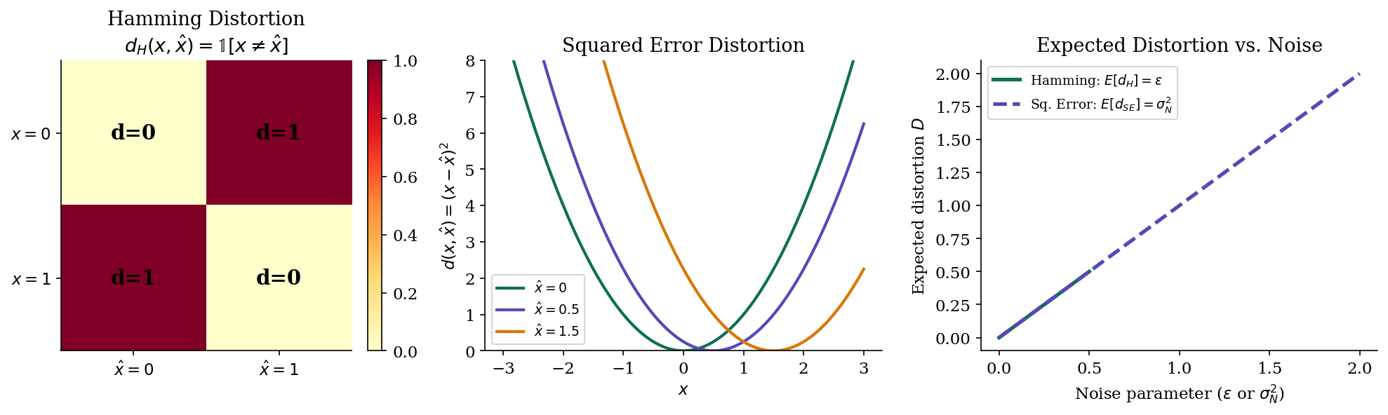
Definition 2 (Hamming Distortion).
For discrete alphabets, the Hamming distortion is
The expected Hamming distortion equals the error probability: .
Definition 3 (Squared Error Distortion).
For real-valued alphabets, the squared error distortion is
The expected squared error distortion is the mean squared error: .
Hamming distortion treats all errors equally — a single bit flip costs the same regardless of context. Squared error, by contrast, is graded: reproducing 3.0 as 3.1 costs far less than reproducing it as 10.0. The choice of distortion measure shapes the entire rate-distortion curve, because it determines what “tolerable” compression means.
For a discrete source with alphabet , the Hamming distortion can be organized into a distortion matrix where . For Hamming distortion, this is simply the identity complement: zeros on the diagonal, ones everywhere else.
The Rate-Distortion Function
The rate-distortion function answers the central question: what is the minimum number of bits per source symbol we need to transmit, if we can tolerate average distortion ?
Definition 4 (Rate-Distortion Function).
For a source with distortion measure , the rate-distortion function is
where the minimization is over all conditional distributions (called test channels) such that the expected distortion .
The test channel describes how we map source symbols to reproductions — it’s the probabilistic encoding rule. The mutual information measures how many bits of information the reproduction carries about the source. Minimizing subject to the distortion constraint finds the most compressed representation that still meets the fidelity requirement.
Proposition 1 (Properties of R(D)).
The rate-distortion function has the following properties:
(i) for all .
(ii) is a non-increasing function of .
(iii) is a convex function of .
(iv) for discrete sources with Hamming distortion (the lossless limit).
(v) for , where is the distortion achievable without any communication.
Proof.
(i) Mutual information is non-negative: , so the minimum is non-negative.
(ii) If , then . Minimizing over a larger set can only decrease (or maintain) the optimum, so .
(iii) Let and lie on the curve, achieved by test channels and respectively. For , the mixture test channel achieves expected distortion . By the convexity of mutual information in for fixed :
(iv) At with Hamming distortion, , so almost surely. Then .
(v) At , we can set (reproduce everything as a constant that minimizes ), achieving .
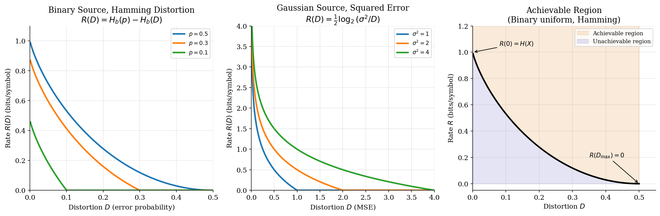
∎Properties (ii) and (iii) together tell us that is a convex, non-increasing curve from down to . The region above the curve is achievable (we can compress to that rate at that distortion); the region below is unachievable (no coding scheme can reach it).
The Rate-Distortion Theorem
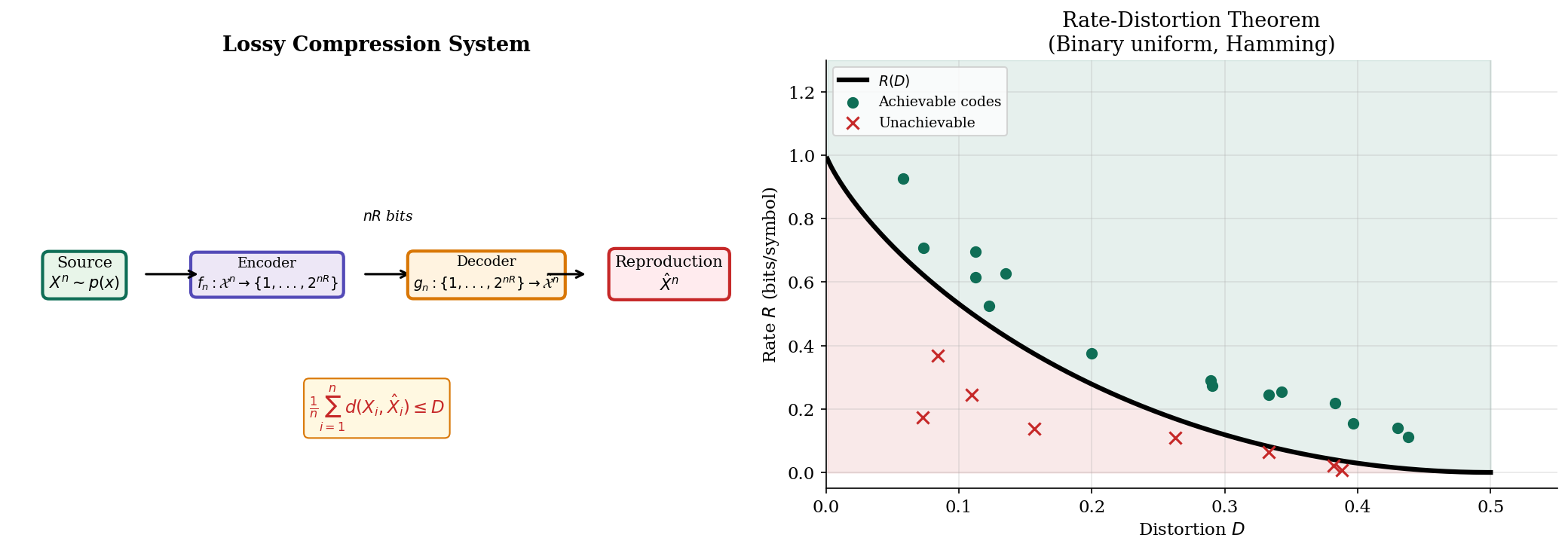
Shannon’s rate-distortion theorem gives its operational meaning: it is the exact boundary between achievable and unachievable compression.
Theorem 3 (Shannon's Rate-Distortion Theorem).
For an i.i.d. source with distortion measure :
Achievability. For any rate , there exists a sequence of codes with expected distortion for all and sufficiently large.
Converse. For any rate , every sequence of codes has expected distortion for sufficiently large.
In other words: bits per symbol are both necessary and sufficient to represent the source with average distortion at most .
Proof.
Achievability. Generate codewords independently from the reproduction distribution induced by the optimal test channel. For a source sequence , find the codeword that is jointly typical with under the optimal test channel.
By the covering lemma, this succeeds with high probability if : we need enough codewords to “cover” the typical set of source sequences. The expected distortion converges to by the properties of jointly typical sequences — each typical pair has per-symbol distortion close to the expected distortion of the test channel.
Converse. By the data processing inequality, for any encoder-decoder pair with index :
For a memoryless source, is independent of , so each conditional mutual information satisfies — conditioning on independent variables cannot increase the information carries about . Therefore .
By the convexity of and Jensen’s inequality applied to the per-symbol distortions :
So , meaning any rate below cannot achieve distortion .
∎The theorem is the operational backbone of lossy compression. The achievability proof is constructive (random coding with joint typicality), while the converse is information-theoretic (any code, no matter how clever, must respect ).
Closed-Form Solutions
For two important source-distortion pairs, has a clean analytical form. These serve as benchmarks and building blocks for understanding the general case.
Binary Source with Hamming Distortion
Theorem 1 (Rate-Distortion for Binary Source).
For a Bernoulli() source with Hamming distortion:
where is the binary entropy function. For , we have .
Proof.
The optimal test channel is a binary symmetric channel BSC(): it flips each bit independently with probability . Under this channel:
- The expected distortion is exactly (the flip probability).
- The mutual information is .
We verify this is optimal by checking the KKT conditions. The Lagrangian is with slope parameter . The optimal test channel satisfies , which for Hamming distortion gives the BSC structure. The distortion constraint is active (), confirming the solution.
At : , recovering lossless compression.
At : , since .
∎For the uniform binary source (), this simplifies to : we start at 1 bit (lossless) and reach 0 bits at (pure guessing).
Gaussian Source with Squared Error
Theorem 2 (Rate-Distortion for Gaussian Source).
For a Gaussian source with squared error distortion:
For , we have .
Proof.
The optimal test channel adds independent Gaussian noise: where is independent of , followed by MMSE estimation . The resulting distortion is exactly .
The mutual information under this channel:
This is optimal because the Gaussian source uniquely achieves the Shannon lower bound (Proposition 2 below) with equality.
At : we can reproduce everything as the mean (zero), achieving zero rate.
∎The Gaussian has a particularly clean interpretation: halving the distortion costs exactly one extra bit per sample. This logarithmic relationship is the foundation of quantization theory.
Parametric Form and the Shannon Lower Bound
Theorem 4 (Parametric Form of R(D)).
The rate-distortion function can be written parametrically via the slope :
where is the optimal test channel at slope , and is its marginal. The slope is the Lagrange multiplier from the Lagrangian dual of the rate-distortion optimization.
For the binary source, the slope parameter is and the test channel is BSC(). For the Gaussian source, , and the test channel adds noise.
Proposition 2 (Shannon Lower Bound).
For any continuous source with differential entropy and squared error distortion:
with equality if and only if is Gaussian. This is the Shannon lower bound (SLB).
Proof.
Starting from the definition:
Since , the conditional entropy is bounded by — because the Gaussian maximizes differential entropy for a given variance. Therefore:
Equality holds when is Gaussian with variance , which happens exactly when itself is Gaussian.
∎The Shannon lower bound tells us that the Gaussian source is the hardest to compress (among sources with the same variance), in the sense that it requires the most bits at every distortion level.

The Blahut–Arimoto Algorithm
For general discrete sources where a closed-form is unavailable, the Blahut–Arimoto (BA) algorithm computes via alternating minimization. The algorithm exploits the convex structure of the rate-distortion optimization.
Theorem 5 (Blahut–Arimoto for Rate-Distortion).
The rate-distortion function for a discrete source with finite alphabet and distortion measure can be computed by the following alternating minimization:
Initialize: .
Repeat until convergence:
Step 1 (Optimize test channel for fixed output marginal):
Step 2 (Update output marginal):
The algorithm converges to the optimal test channel for the given slope . Sweeping from to traces out the entire curve.
Proof.
The Lagrangian of the rate-distortion optimization is
This decomposes into two subproblems when we alternate between optimizing the test channel and the output marginal . Each step decreases :
- Step 1 minimizes over for fixed . The solution is the Gibbs distribution , obtained by setting the functional derivative to zero.
- Step 2 minimizes over for fixed . The optimal is the marginal , which minimizes the KL divergence .
Since is bounded below and decreases at each step, the algorithm converges. Since the original problem is convex, the limit is the global optimum.
∎The connection to the EM algorithm is direct: Step 1 is analogous to the E-step (computing a posterior given current parameters), and Step 2 is analogous to the M-step (updating parameters given the posterior). Both algorithms exploit the same alternating minimization structure on convex objectives.
Here is the Python implementation:
def blahut_arimoto_rd(px, distortion_matrix, slope, max_iter=200, tol=1e-10):
    """Blahut-Arimoto for one point on the R(D) curve."""
    n_x, n_xhat = distortion_matrix.shape
    q_xhat = np.ones(n_xhat) / n_xhat  # uniform initialization

    for iteration in range(max_iter):
        # Step 1: optimal test channel
        log_channel = np.log(np.maximum(q_xhat, 1e-300)) + slope * distortion_matrix
        log_channel -= log_channel.max(axis=1, keepdims=True)
        p_xhat_given_x = np.exp(log_channel)
        p_xhat_given_x /= p_xhat_given_x.sum(axis=1, keepdims=True)

        # Step 2: update output marginal
        new_q = px @ p_xhat_given_x
        new_q = np.maximum(new_q, 1e-300)

        if np.max(np.abs(new_q - q_xhat)) < tol:
            break
        q_xhat = new_q

    # Compute rate and distortion
    joint = px[:, None] * p_xhat_given_x
    rate = mutual_information(joint)
    distortion = np.sum(joint * distortion_matrix)
    return rate, distortion, q_xhat, p_xhat_given_x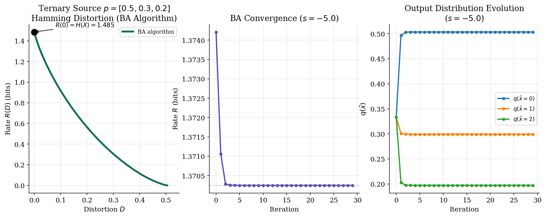
The Information Bottleneck
The information bottleneck (IB) method, introduced by Tishby, Pereira & Bialek (1999), extends rate-distortion theory from compression of to compression of while preserving information about a relevant variable . This is the bridge between rate-distortion theory and representation learning.
Definition 5 (Information Bottleneck).
Given a joint distribution , the information bottleneck seeks a compressed representation of that maximizes information about . The IB Lagrangian is
where controls the compression-relevance trade-off:
- = complexity — how much we remember about
- = relevance — how much tells us about
- = Lagrange multiplier: large favors relevance, small favors compression
The IB is not just an abstract optimization — it is a special case of rate-distortion theory with an information-theoretic distortion measure.
Proposition 3 (IB as Rate-Distortion with KL Distortion).
The IB problem is equivalent to a rate-distortion problem with the “log-loss” distortion measure:
The “cost” of representing by is the KL divergence between their conditional distributions over . This makes the IB a special case of rate-distortion theory where the distortion is information-theoretic.
Proof.
We want to minimize subject to . Using the Markov chain (the representation depends on only through ), we proceed in three steps.
Step 1: Decompose the relevance constraint. Write mutual information as a conditional entropy difference:
So is equivalent to .
Step 2: Introduce the KL distortion. By the Markov chain , we have . The gap between conditional entropies decomposes as:
where is the KL distortion measure. This is non-negative (by Gibbs’ inequality) and equals zero only when preserves the full conditional .
Step 3: Reformulate as rate-distortion. Since is a constant of the source, the constraint becomes for . The IB objective subject to this expected distortion constraint is exactly the rate-distortion problem with the distortion measure .
∎Proposition 4 (IB Curve Properties).
The IB curve — the set of achievable pairs — has the following properties:
(i) It is a concave function of .
(ii) when (no compression implies no relevance).
(iii) when (perfect representation preserves all relevance).
(iv) The slope at any point equals .
The IB curve tells us exactly how much relevance we must sacrifice for each bit of compression. Low means heavy compression (small , low relevance); high means preserving relevance at the cost of a more complex representation.
def information_bottleneck(p_xy, beta, n_t=4, max_iter=500, tol=1e-10):
    """Compute IB solution for given beta via alternating optimization."""
    n_x, n_y = p_xy.shape
    p_x = p_xy.sum(axis=1)
    p_y_given_x = p_xy / p_x[:, None]

    # Initialize p(t|x) randomly
    p_t_given_x = np.random.dirichlet(np.ones(n_t), size=n_x)

    for _ in range(max_iter):
        p_t = p_x @ p_t_given_x
        p_t = np.maximum(p_t, 1e-300)

        # p(y|t) from Bayes: p(y|t) = sum_x p(y|x) p(x|t)
        p_y_given_t = np.zeros((n_t, n_y))
        for t in range(n_t):
            if p_t[t] > 1e-300:
                p_y_given_t[t] = (p_t_given_x[:, t] * p_x) @ p_y_given_x / p_t[t]

        # Update p(t|x) proportional to p(t) exp(-beta * D_KL(p(y|x) || p(y|t)))
        new_p = np.zeros_like(p_t_given_x)
        for i in range(n_x):
            for t in range(n_t):
                dkl = np.sum(
                    p_y_given_x[i] * np.log(
                        np.maximum(p_y_given_x[i], 1e-300)
                        / np.maximum(p_y_given_t[t], 1e-300)
                    ) * (p_y_given_x[i] > 0)
                )
                new_p[i, t] = p_t[t] * np.exp(-beta * dkl)
            new_p[i] /= np.maximum(new_p[i].sum(), 1e-300)

        if np.max(np.abs(new_p - p_t_given_x)) < tol:
            break
        p_t_given_x = new_p

    # Compute I(X;T) and I(T;Y)
    p_xt = p_x[:, None] * p_t_given_x
    I_XT = mutual_information(p_xt)
    p_ty = np.diag(p_t) @ p_y_given_t
    I_TY = mutual_information(p_ty)
    return I_XT, I_TY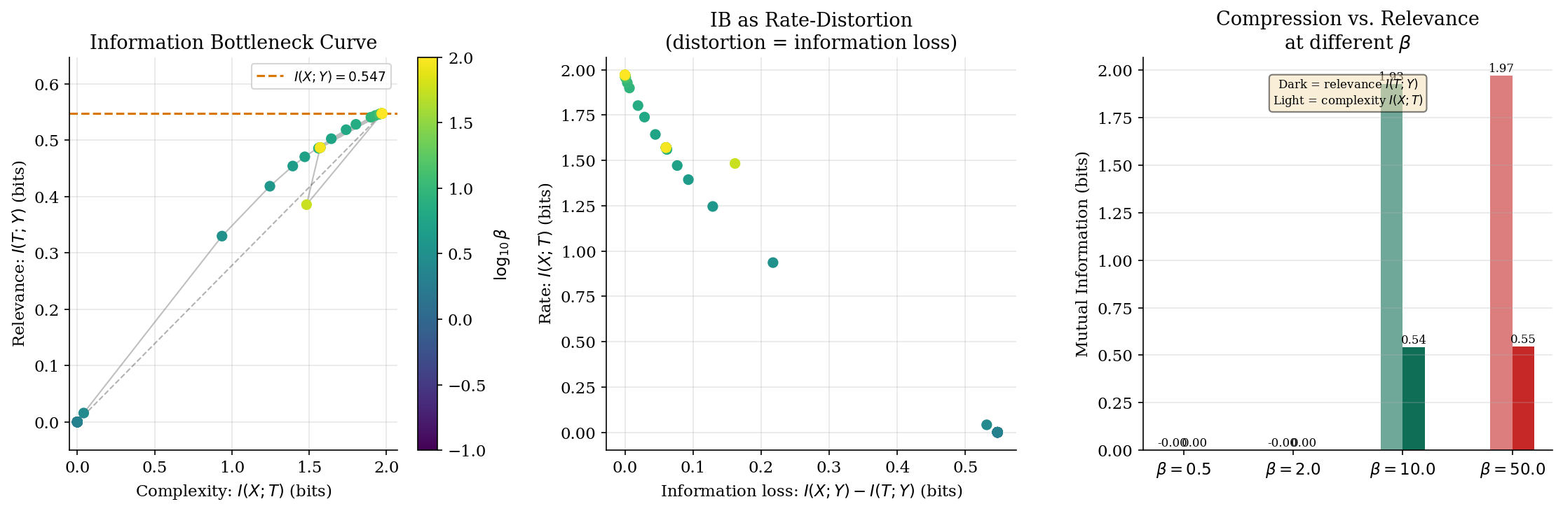
Data Processing and Successive Refinement
Two additional results connect rate-distortion theory to practical coding systems.
Proposition 5 (DPI and Rate-Distortion).
For the Markov chain (post-processing the compressed representation):
by the data processing inequality. Since is non-increasing, post-processing cannot improve the rate-distortion trade-off: it can only increase distortion or maintain it (if the processing is sufficient statistic-preserving).
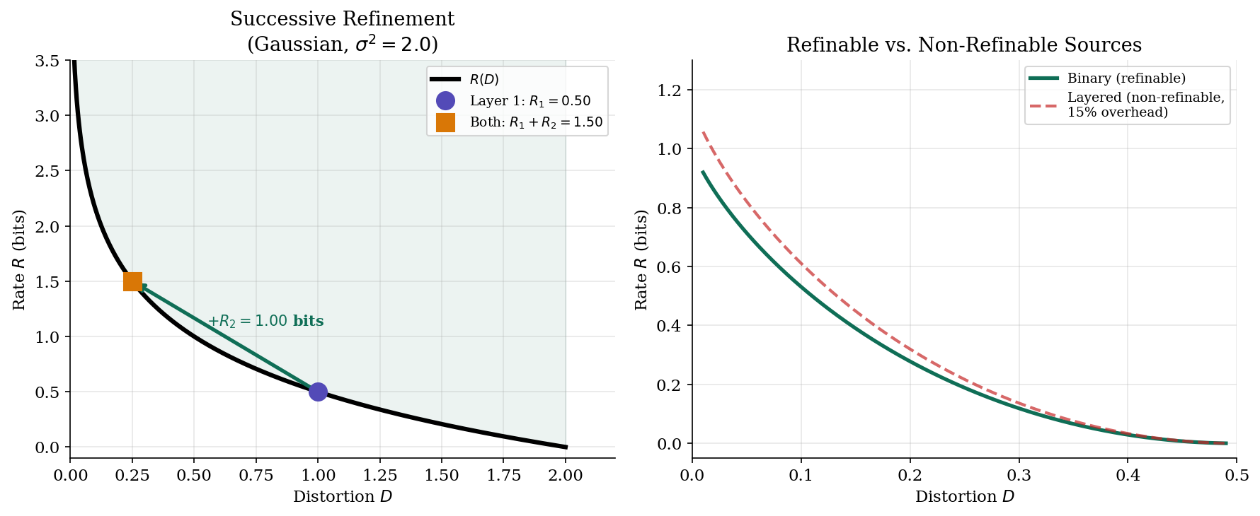
Proposition 6 (Successive Refinement).
A source is successively refinable if the rate-distortion curve can be achieved by layered coding: a first description at rate achieves distortion , and a second description at rate (given the first) achieves distortion , such that:
Theorem (Equitz & Cover, 1991): A source is successively refinable if and only if the optimal test channels at and form a Markov chain . The Gaussian source with squared error is successively refinable.
Successive refinement is the theoretical foundation of progressive coding (JPEG progressive, scalable video coding): a base layer provides coarse quality, and enhancement layers refine it without wasting bits.
Computational Notes
Rate-distortion theory connects directly to modern ML through three bridges: the VAE loss, neural compression, and the information bottleneck in deep learning.
VAE Loss as Rate-Distortion
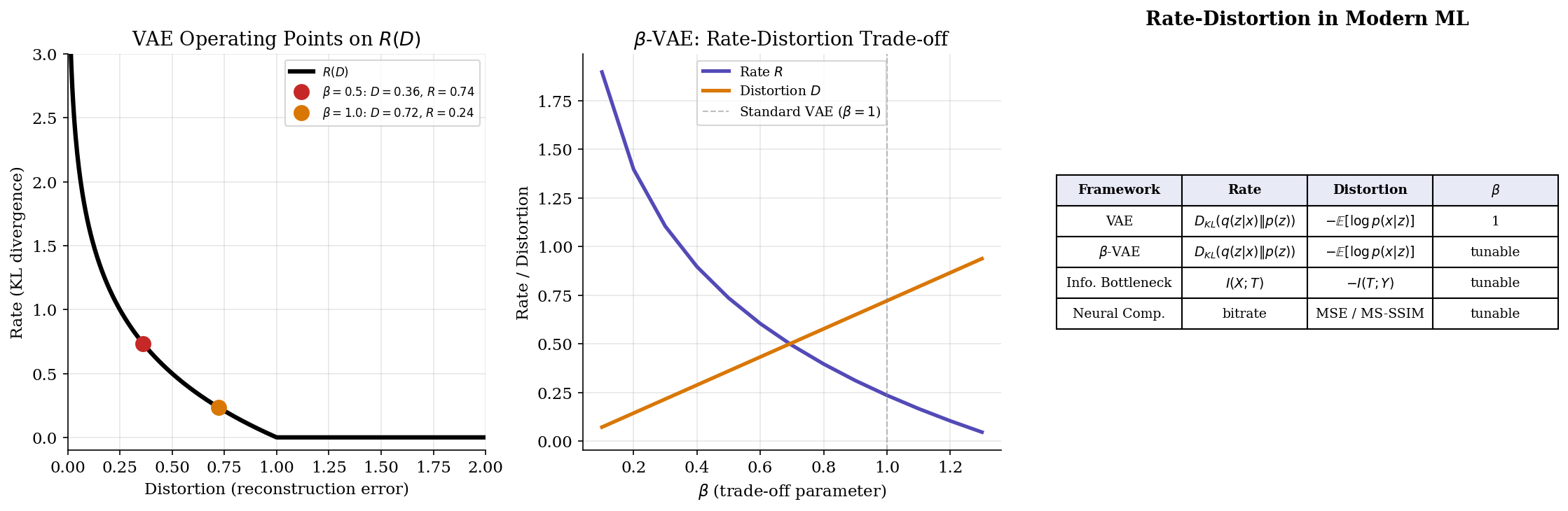
Remark (VAE Loss as Rate-Distortion).
The VAE objective (ELBO) can be written as:
This is precisely the rate-distortion Lagrangian with (standard VAE). The reconstruction term is the distortion (negative log-likelihood under the decoder), and the KL term is the rate (complexity of the latent code).
Remark (β-VAE and Rate-Distortion Trade-off).
The -VAE (Higgins et al., 2017) modifies the ELBO with a tunable :
This traces the rate-distortion curve:
- : prioritize reconstruction (low distortion, high rate)
- : prioritize compression (low rate, higher distortion, more disentangled representations)
- : standard VAE (the “natural” operating point on the R(D) curve)
Python Implementations
Here are reference implementations for computing rate-distortion functions:
def rate_distortion_binary(p, D):
    """R(D) = H_b(p) - H_b(D) for binary source with Hamming distortion."""
    D_max = min(p, 1 - p)
    if D >= D_max:
        return 0.0
    return H_b(p) - H_b(D)

def rate_distortion_gaussian(sigma2, D):
    """R(D) = 0.5 * log2(sigma2 / D) for Gaussian source."""
    if D >= sigma2:
        return 0.0
    return 0.5 * np.log2(sigma2 / D)
# VAE loss decomposition
def vae_loss(x, encoder, decoder, beta=1.0):
"""L = E[-log p(x|z)] + β D_KL(q(z|x) || p(z))"""
mu, logvar = encoder(x)
z = reparameterize(mu, logvar)
# Distortion: reconstruction error
recon_loss = -decoder.log_prob(x, z).mean()
# Rate: KL divergence from posterior to prior
kl_loss = -0.5 * (1 + logvar - mu**2 - logvar.exp()).sum(dim=-1).mean()
return recon_loss + beta * kl_loss # rate-distortion LagrangianNeural Compression
Modern learned image and video codecs operationalize rate-distortion theory directly. The encoder-decoder architecture learns the optimal test channel end-to-end, with the loss function being exactly the rate-distortion Lagrangian:
where is the quantized latent representation and is the learned entropy model. Different values trace out the operational R(D) curve of the neural codec. Frameworks like CompressAI (Ballé et al.) achieve state-of-the-art image compression by learning both the transform and the entropy model jointly.
Connections & Further Reading
Connection Map
-
Shannon Entropy & Mutual Information — : the rate-distortion function is defined as a minimization of mutual information. At , recovers the lossless source coding limit.
-
KL Divergence & f-Divergences — The KL divergence appears in the IB distortion measure and in the VAE rate term .
-
Convex Analysis — is convex in : the rate-distortion optimization is a convex program. The Blahut–Arimoto algorithm exploits this structure via alternating minimization.
-
Lagrangian Duality & KKT — The slope in the parametric form of is the Lagrange multiplier for the distortion constraint. Strong duality holds because the optimization is convex.
-
Minimum Description Length — MDL connects source coding (Shannon) to model selection: the best model minimizes description length = code length + model complexity.
Notation Reference
| Symbol | Meaning |
|---|---|
| Distortion function: cost of reproducing as | |
| Expected (average) distortion | |
| Rate-distortion function: minimum bits/symbol at distortion | |
| Test channel: conditional distribution from source to reproduction | |
| Maximum useful distortion: achievable without any communication | |
| Slope parameter (Lagrange multiplier) in the parametric form | |
| Trade-off parameter in IB / -VAE | |
| Complexity (compression) in the information bottleneck | |
| Relevance (preserved information) in the information bottleneck |
Connections
- R(D) = min I(X; X̂) — the rate-distortion function minimizes mutual information. At D = 0, R(0) = H(X) recovers the lossless source coding limit established by the source coding theorem. shannon-entropy
- The information bottleneck distortion measure is d_IB(x, t) = D_KL(p(y|x) || p(y|t)), and the VAE rate term is D_KL(q(z|x) || p(z)). Both bridge rate-distortion theory to modern ML. kl-divergence
- R(D) is convex in D — the rate-distortion optimization is a convex program. The Blahut–Arimoto algorithm exploits convexity via alternating minimization, and Lagrangian duality gives the parametric form. convex-analysis
- The slope parameter s in the parametric form of R(D) is the Lagrange multiplier for the distortion constraint. Strong duality holds because the optimization is convex. The KKT conditions yield the optimal test channel structure. lagrangian-duality
References & Further Reading
- book Elements of Information Theory — Cover & Thomas (2006) Chapters 10–13 — rate-distortion theory, closed-form solutions, Blahut–Arimoto algorithm
- book Rate Distortion Theory: A Mathematical Basis for Data Compression — Berger (1971) The classical monograph on rate-distortion theory
- paper Computation of Channel Capacity and Rate-Distortion Functions — Blahut (1972) The original Blahut–Arimoto algorithm for computing R(D) via alternating minimization
- paper The Information Bottleneck Method — Tishby, Pereira & Bialek (1999) Introduction of the information bottleneck — rate-distortion with relevance
- paper Deep Variational Information Bottleneck — Alemi, Fischer, Dillon & Murphy (2017) Connects the information bottleneck to deep learning via variational bounds
- paper β-VAE: Learning Basic Visual Concepts with a Constrained Variational Framework — Higgins, Matthey, Pal, Burgess, Glorot, Botvinick, Mohamed & Lerchner (2017) β-VAE as rate-distortion trade-off — tuning β traces the R(D) curve