Lagrangian Duality & KKT Conditions
The Lagrangian, weak and strong duality, Slater's condition, KKT optimality conditions, sensitivity analysis, and applications to SVMs, water-filling, and portfolio optimization
Overview & Motivation
In Convex Analysis we developed the foundations — convex sets, convex functions, subdifferentials, and the separation theorems. In Gradient Descent & Convergence and Proximal Methods we built algorithms for unconstrained optimization (or at least for objectives where constraints could be absorbed into the proximal operator). But many of the most important problems in machine learning and engineering are constrained: minimize an objective subject to explicit limits on the variables.
Consider training a support vector machine. We want the widest-margin separating hyperplane, but we require that every training point lies on the correct side of the boundary. Or consider allocating power across communication channels: we want to maximize total capacity, but we have a fixed total power budget. Or consider building a portfolio: we want maximum expected return, but we can’t exceed a given risk tolerance.
The direct approach — “optimize over the feasible set” — is often intractable. The feasible set might have a complicated geometry, or the constraints might couple variables in ways that make projection expensive. Lagrangian duality offers an alternative: attach a price (a dual variable, or multiplier) to each constraint, fold the constraints into the objective, and solve an unconstrained problem instead. The dual variables play a double role: they enforce the constraints at optimality, and they measure the sensitivity of the optimal value to constraint perturbations.
The punchline is the KKT conditions — four equations that are necessary and sufficient for optimality in convex programs. When you see a machine learning paper derive a closed-form solution to a constrained problem, the KKT conditions are almost always the tool that gets them there.
What We Cover
- The Lagrangian & Dual Problem — the Lagrangian function, dual variables as prices on constraint violations, the dual function as a pointwise infimum, and concavity of the dual.
- Weak Duality — the universal inequality and the duality gap.
- Strong Duality & Slater’s Condition — when the gap closes to zero, and the geometric picture via the perturbation function.
- KKT Conditions — stationarity, primal feasibility, dual feasibility, and complementary slackness; necessity under strong duality and sufficiency for convex programs.
- Complementary Slackness — the economic insight: you only pay for constraints that bind.
- Saddle Point Interpretation — the minimax theorem and the Lagrangian as a saddle surface.
- Sensitivity Analysis — shadow prices, the perturbation function, and the identity .
- Application: The SVM Dual — the hard-margin SVM, the kernel trick as a consequence of duality, and support vectors via complementary slackness.
- Application: Water-Filling & Portfolio Optimization — KKT in closed form for channel capacity and the efficient frontier.
- Computational Notes — CVXPY with dual extraction, scipy SLSQP, and the barrier method.
The Lagrangian & Dual Problem
We start with the standard form of a constrained convex optimization problem.
Definition 1 (Standard Form Convex Program).
A standard form convex program is
where are convex functions and are affine functions (). The primal optimal value is .
The affineness requirement on the equality constraints is not a minor technicality — it’s what keeps the feasible set convex. A nonlinear equality constraint generally defines a non-convex surface, which would destroy the convexity of the problem.
Now we introduce the central object: the Lagrangian function. The idea is to relax the hard constraints into a penalty term weighted by dual variables.
Definition 2 (The Lagrangian Function).
The Lagrangian associated with the standard form problem is the function defined by
where with are the dual variables (or Lagrange multipliers) for the inequality constraints, and are the dual variables for the equality constraints.
Think of as a price on violating the -th constraint. When (the constraint is violated), the term adds a positive penalty to the objective. When (the constraint has slack), the term is negative — it rewards having extra room. The dual variable controls how aggressively we penalize violations.
Now we minimize the Lagrangian over to obtain a function of the dual variables alone.
Definition 3 (The Lagrange Dual Function).
The Lagrange dual function is
The dual problem is
with dual optimal value .
The dual function has a remarkable structural property that does not depend on convexity of the primal problem.
Proposition 1 (Concavity of the Dual Function).
The dual function is concave, even if the primal problem is not convex. Consequently, the dual problem is always a concave maximization problem.
Proof.
For any fixed , the function is affine (and hence concave) in . The dual function is the pointwise infimum of a family of affine functions. Since the pointwise infimum of any collection of concave functions is concave, is concave.
∎This is a powerful result. No matter how ugly the primal problem is — non-convex objective, non-convex constraints, disconnected feasible set — the dual is always a concave maximization. The dual is a “convexification” of the primal, and it always produces useful lower bounds.
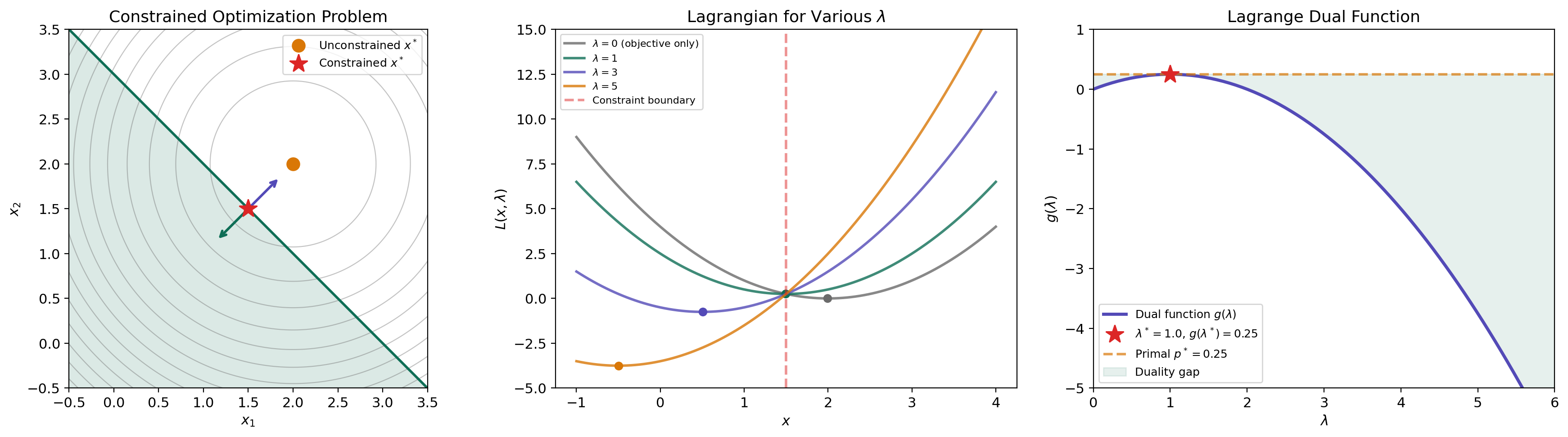
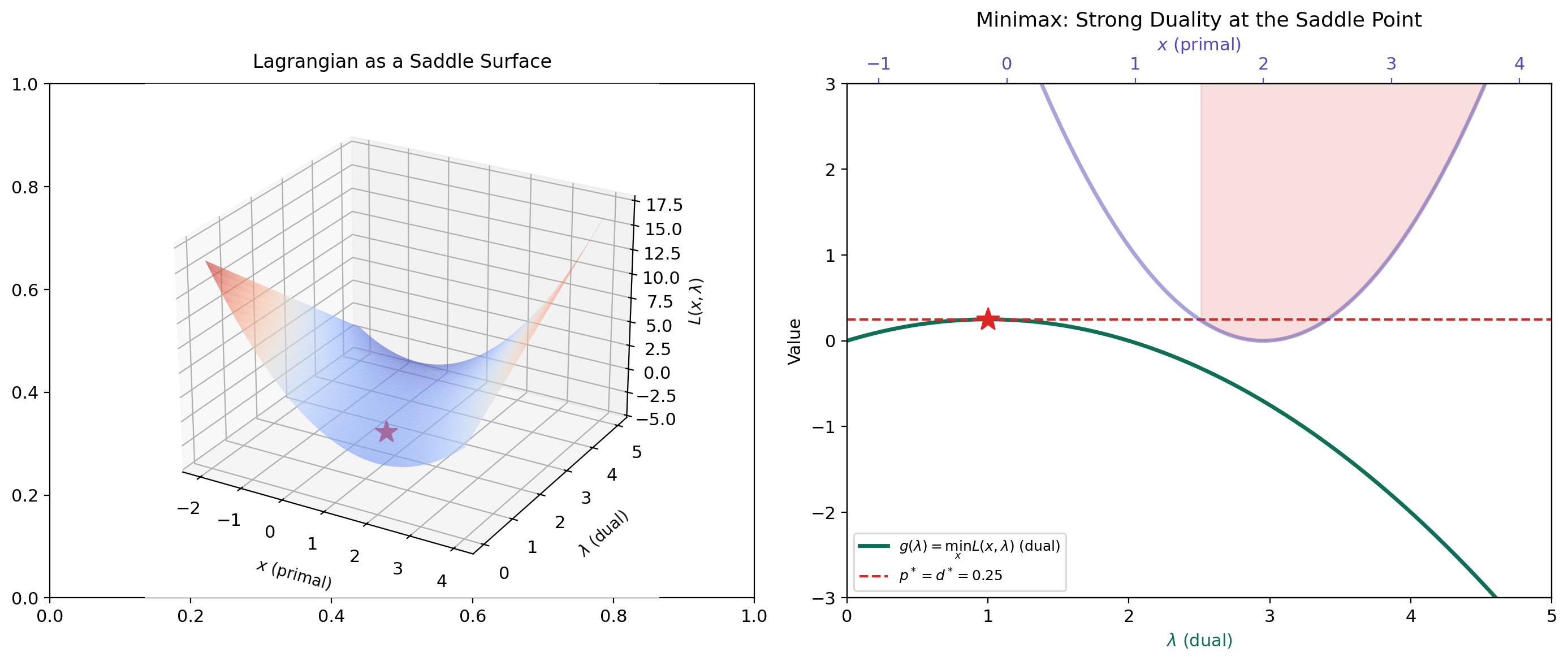
A concrete example. Consider minimizing subject to (i.e., ). The Lagrangian is . Minimizing over (take the derivative, set to zero): , so . Substituting back:
This is a concave quadratic in , maximized at with . The primal optimum is , so — strong duality holds.
p* = 2.2500 | g(λ=2.0) = 2.0000 | gap = 0.2500
Weak Duality
The most fundamental inequality in optimization theory requires almost no assumptions.
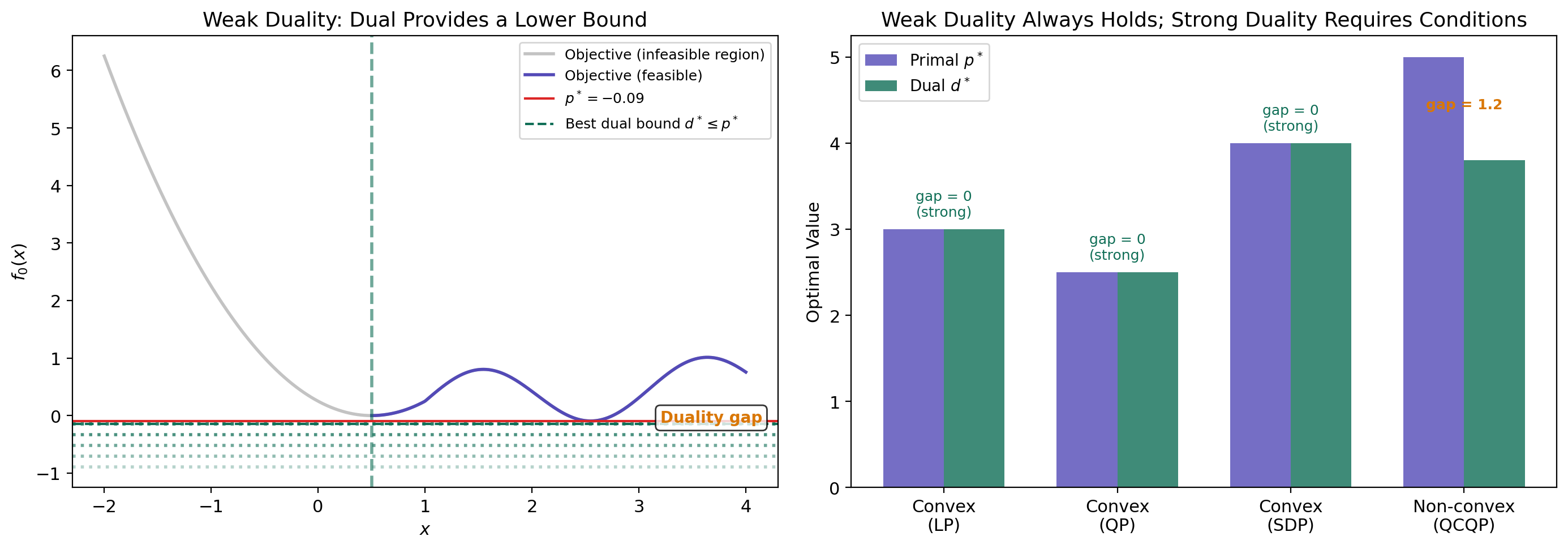
Theorem 1 (Weak Duality).
For any optimization problem (not necessarily convex), the dual optimal value lower-bounds the primal optimal value:
More precisely, for any primal-feasible and any dual-feasible with :
The difference is called the duality gap.
Proof.
Let be primal-feasible (so for all and for all ) and let be dual-feasible (so ). Then:
The first inequality holds because the infimum over all is at most the value at a particular . The second inequality uses and (so each product is non-positive) and . Since this holds for all primal-feasible and dual-feasible , taking the supremum over dual variables and infimum over primal variables gives .
∎The proof is elegantly simple — just two inequalities and a sign argument. Note that we never used convexity. Weak duality holds for arbitrary optimization problems: non-convex objectives, non-convex constraints, discrete variables, anything. This universality is what makes the dual function so useful as a bounding tool even when we can’t solve the primal exactly.
The duality gap measures how much information we lose by passing to the dual. For non-convex problems, the gap can be strictly positive — the dual relaxation is too loose. The central question is: when does the gap close?
Strong Duality & Slater’s Condition
Strong duality — the statement that — is the bridge that makes the dual problem as powerful as the primal. It holds for convex problems under a mild regularity condition.
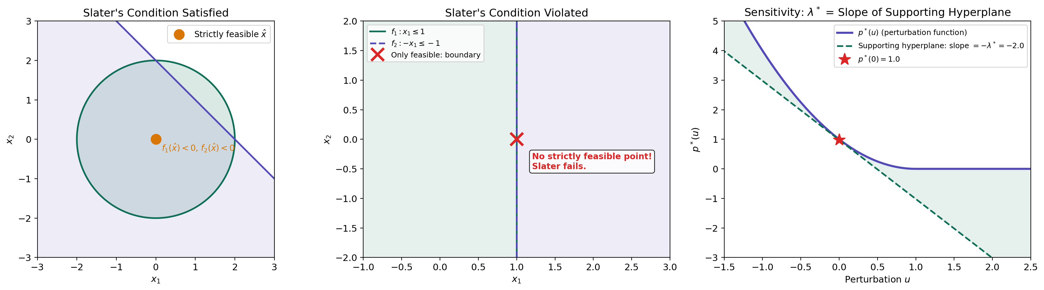
Definition 4 (Slater's Condition).
A convex program satisfies Slater’s condition (or is Slater-qualified) if there exists a point in the relative interior of the feasible set such that
That is, there exists a strictly feasible point — one that satisfies all inequality constraints with strict inequality.
Slater’s condition is saying that the feasible set has a non-empty interior (it’s not “infinitely thin”). The inequality constraints must have room to breathe — you can’t have the feasible set consist entirely of points where some constraint is active. The equality constraints, being affine, must still be satisfied exactly.
Theorem 2 (Strong Duality (Slater)).
If a convex program satisfies Slater’s condition and the primal optimal value is finite, then strong duality holds:
Moreover, the dual optimum is attained: there exist and such that .
Proof.
We prove this via the separating hyperplane theorem applied to the perturbation set. Define the set
This is a convex set (because are convex and are affine). The primal optimal value corresponds to the point : the best objective value achievable when no constraint is perturbed.
Consider the point for any . This point lies outside (because is optimal — we can’t do better). By the supporting hyperplane theorem (from Convex Analysis), there exists a hyperplane separating from . Taking , we obtain a supporting hyperplane at .
The normal to this hyperplane gives us the dual variables: with and . The separating hyperplane condition gives, for all :
Slater’s condition ensures (the hyperplane is not vertical — it has a non-trivial component in the -direction). Dividing by and rearranging, this gives . Combined with weak duality , we conclude .
∎When Slater fails. If the feasible set has no interior — for example, if the inequality constraints all hold with equality — then the separating hyperplane might be vertical (), and the dual may not recover the primal value. A concrete example: minimize subject to . The only feasible point is , so . The dual function is . For any finite , the infimum is driven toward zero as (the exponential decays faster than the quadratic grows for any fixed ), so for all . Hence — a positive duality gap, because the feasible set is a single point with no interior.
LP strong duality. For linear programs, strong duality holds without Slater’s condition — the LP duality theorem guarantees whenever the primal is feasible and bounded. This is because the Lagrangian is linear in , so the infimum is either or attained at a vertex.
KKT Conditions
The Karush–Kuhn–Tucker conditions are the first-order necessary and sufficient conditions for optimality in convex programs with strong duality. They are the constrained analogue of the unconstrained condition .
Definition 5 (Karush–Kuhn–Tucker (KKT) Conditions).
A primal-dual triple satisfies the KKT conditions for the standard form convex program if all four of the following hold:
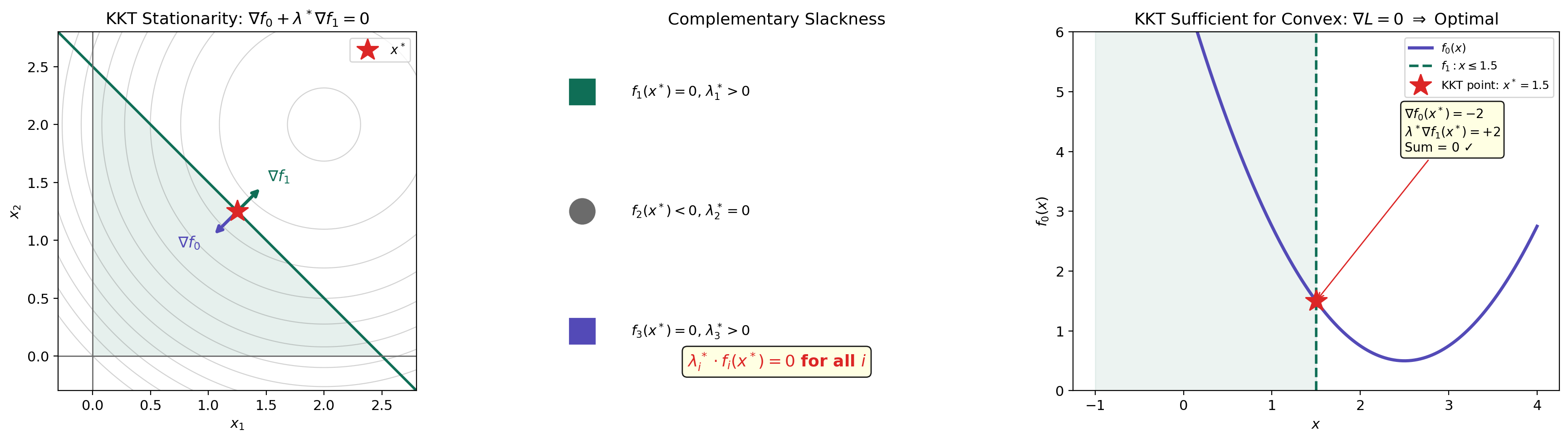
- Stationarity:
- Primal feasibility: for all and for all
- Dual feasibility: for all
- Complementary slackness: for all
Stationarity says that the gradient of the Lagrangian with respect to vanishes at the optimum — the objective gradient is cancelled by a non-negative combination of the constraint gradients. Geometrically, lies in the cone spanned by the active constraint gradients .
Theorem 3 (KKT Necessary Conditions).
If strong duality holds (i.e., and the dual optimum is attained), and is primal-optimal and is dual-optimal, then satisfies the KKT conditions.
Proof.
Since is primal-optimal and is dual-optimal, and strong duality holds:
We also know (from the weak duality proof) that
The last inequality uses , , and . Since the left and right sides are equal (both equal ), every inequality in the chain must hold with equality.
Complementary slackness: The equality with each term forces for each .
Stationarity: The equality means minimizes . Since the Lagrangian is convex in (as a sum of convex functions weighted by non-negative coefficients plus affine functions), the first-order condition gives , which is exactly the stationarity condition.
Primal and dual feasibility hold by assumption ( is primal-feasible, ).
∎The converse is even more powerful for convex problems.
Theorem 4 (KKT Sufficient for Convex Programs).
For a convex program, if satisfies the KKT conditions, then is primal-optimal, is dual-optimal, and strong duality holds with zero duality gap.
Proof.
Suppose the KKT conditions hold. Stationarity means minimizes over (since for a convex function, implies global minimum). Therefore:
So . By weak duality, . But . Therefore : strong duality holds, is primal-optimal, and is dual-optimal.
∎Together, Theorems 3 and 4 give the complete picture for convex programs with Slater’s condition: the KKT conditions are necessary and sufficient for optimality. This is the constrained analogue of “set the gradient to zero and solve.”
KKT Conditions
Drag the point to explore KKT conditions at different locations.
Complementary Slackness
Complementary slackness deserves special attention because it is the condition that does the most work in applications.
Theorem 5 (Complementary Slackness).
If strong duality holds and is a primal-dual optimal pair, then for each inequality constraint :
That is, either (the multiplier is zero — the constraint is “free”) or (the constraint is active — it holds with equality). Both can be zero simultaneously, but they cannot both be strictly positive/negative.
Proof.
This was established in the proof of Theorem 3. The chain of equalities forces . Since each term satisfies and , each product . A sum of non-positive terms equals zero only if each term is zero.
∎The economic interpretation is clean: is the price you’re paying for constraint . If the constraint has slack ( — you have unused capacity), the price is zero — you wouldn’t pay anything to relax a constraint that isn’t binding. If the constraint is active ( — you’re at the limit), then the multiplier tells you how much the optimal value would improve per unit of relaxation.
This insight is what identifies the support vectors in an SVM: the data points where the margin constraint is active () are exactly the ones that determine the decision boundary. All other points have and can be removed without changing the solution.
Saddle Point Interpretation
The KKT conditions have an elegant reformulation in terms of saddle points of the Lagrangian.
Definition 6 (Saddle Point of the Lagrangian).
A point with is a saddle point of the Lagrangian if
for all , all , and all . That is, minimizes and maximizes it.
The Lagrangian is a “game” between two players. The primal player chooses to minimize ; the dual player chooses to maximize it. At a saddle point, neither player can improve their position unilaterally. This is the minimax interpretation:
When strong duality holds, the max and min commute — the order of play doesn’t matter. This is the minimax theorem applied to the Lagrangian.
Theorem 6 (Saddle Point Equivalence).
For a convex program, is a saddle point of if and only if is primal-optimal, is dual-optimal, and strong duality holds.
Proof.
() Suppose is a saddle point. The right inequality for all means minimizes , so .
The left inequality for all and . Taking : . The maximization over of the left side, evaluated at feasible, forces to be primal-feasible (otherwise we could make ). With feasible: , giving zero duality gap.
() If , are primal and dual optimal with zero gap, then KKT holds (Theorem 3). Stationarity gives the right inequality; the left inequality follows because for feasible , is maximized at by complementary slackness.
∎L(1.50, 3.00) = 2.2500 | Saddle point: L(1.5, 3) = 2.2500 ← you are at the saddle point!
Sensitivity Analysis
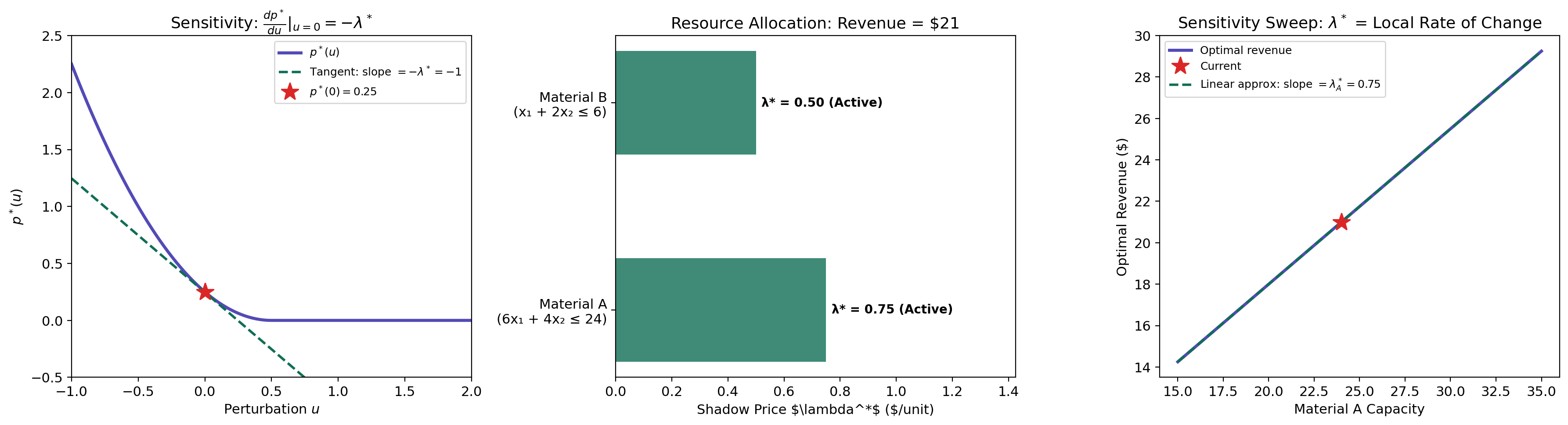
Dual variables are not just abstract quantities needed to state the KKT conditions — they have a concrete interpretation as shadow prices that measure how sensitive the optimal value is to constraint perturbations.
Theorem 7 (Sensitivity via Dual Variables).
Consider the perturbed problem: minimize subject to and , with optimal value . If strong duality holds and the dual optimum is attained for the unperturbed problem (), then
That is, the optimal dual variable is the shadow price of constraint : it measures the rate at which the optimal value decreases when the constraint is relaxed.
Proof.
The dual function for the perturbed problem is
By strong duality for the perturbed problem (assuming Slater holds for small perturbations):
At : , and the maximizer is . By the envelope theorem (the derivative of the optimum with respect to a parameter equals the partial derivative of the objective at the optimal point):
The same argument gives .
∎The sign makes economic sense. A positive means the constraint is active and costly. Increasing (relaxing the constraint to ) gives more room, which decreases the optimal objective by approximately per unit of relaxation. A large shadow price means the constraint is bottleneck — relaxing it yields large improvements.
Resource allocation example. Suppose a factory maximizes profit subject to material constraints. If the shadow price of steel is $7.50/kg and the shadow price of copper is $0/kg, then buying one more kilogram of steel improves profit by $7.50, while copper has slack — the current supply isn’t a binding limit. This tells the manager exactly where to invest.
p*(0) = -3.0000 | p*(0.00) = -3.0000 | Δp* ≈ −λ*·u = −0.75×0.00 = 0.0000
Application: The SVM Dual
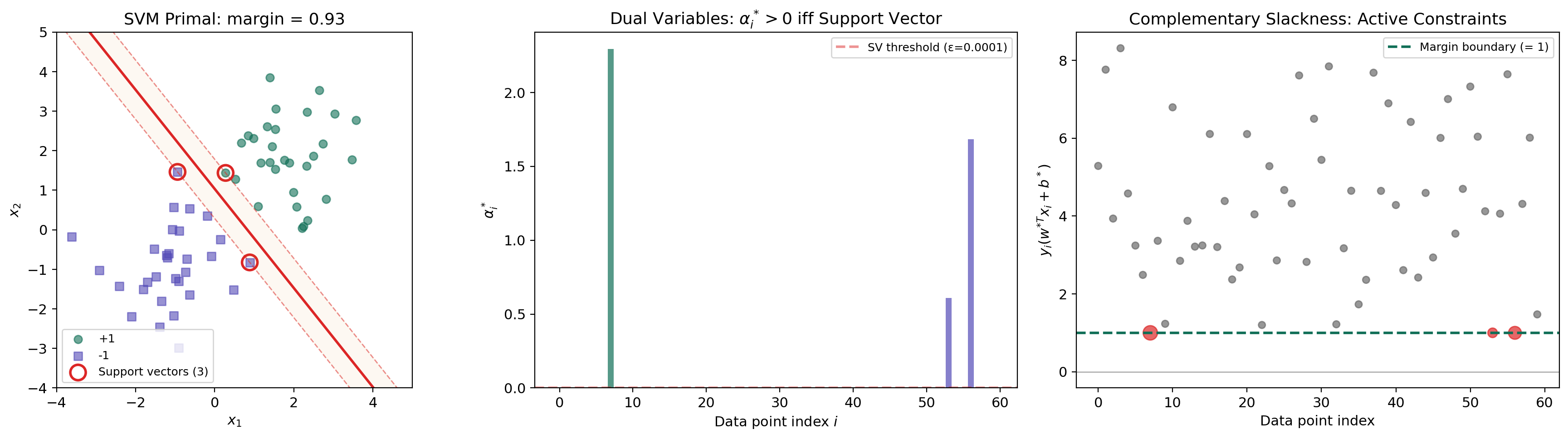
The hard-margin support vector machine is perhaps the most celebrated application of Lagrangian duality in machine learning. The dual formulation reveals the kernel trick, identifies the support vectors via complementary slackness, and reduces the problem to a tractable QP.
The primal. Given linearly separable training data with and , the hard-margin SVM solves:
The objective minimizes , which maximizes the margin . The constraints require each point to be on the correct side of the margin.
The Lagrangian. Introducing multipliers for each constraint:
KKT stationarity. Setting the gradient of with respect to and to zero:
The first equation is remarkable: the optimal weight vector is a linear combination of the training points, weighted by the dual variables. Only points with contribute — these are the support vectors.
The dual QP. Substituting the stationarity conditions back into the Lagrangian:
Remark (Why the SVM Dual Reveals the Kernel Trick).
The dual objective depends on the data only through the inner products . This means we can replace with a kernel function — computing inner products in a high-dimensional (even infinite-dimensional) feature space without ever explicitly mapping the data. This is the kernel trick, and it is a direct consequence of the dual formulation. The primal objective depends on explicitly, which lives in the feature space — the kernel trick would not be visible from the primal alone.
Complementary slackness identifies support vectors. By complementary slackness, for each . Either (the point doesn’t contribute to ) or (the point lies exactly on the margin). Points with are the support vectors — they sit on the margin boundary and fully determine the classifier. All other points could be removed without changing the solution.
import numpy as np
from scipy.optimize import minimize as sp_minimize

def svm_dual(X, y):
    """Solve the hard-margin SVM dual via scipy."""
    n = X.shape[0]
    Q = np.outer(y, y) * (X @ X.T)  # Gram matrix

    def neg_dual(alpha):
        return -np.sum(alpha) + 0.5 * alpha @ Q @ alpha

    def neg_dual_grad(alpha):
        return -np.ones(n) + Q @ alpha

    constraints = [{'type': 'eq', 'fun': lambda a: a @ y}]
    bounds = [(0, None)] * n
    result = sp_minimize(neg_dual, np.zeros(n), jac=neg_dual_grad,
                         bounds=bounds, constraints=constraints, method='SLSQP')
    alpha = result.x

    # Recover w* = sum alpha_i y_i x_i
    w = (alpha * y) @ X
    # Recover b* from a support vector
    sv = np.where(alpha > 1e-6)[0]
    b = np.mean(y[sv] - X[sv] @ w)
return w, b, alphaSupport vectors: 12 / 20 | margin = 3.0335 | w = [0.394, 0.528], b = -0.491
Application: Water-Filling & Portfolio Optimization
Two more applications where the KKT conditions yield closed-form or near-closed-form solutions.
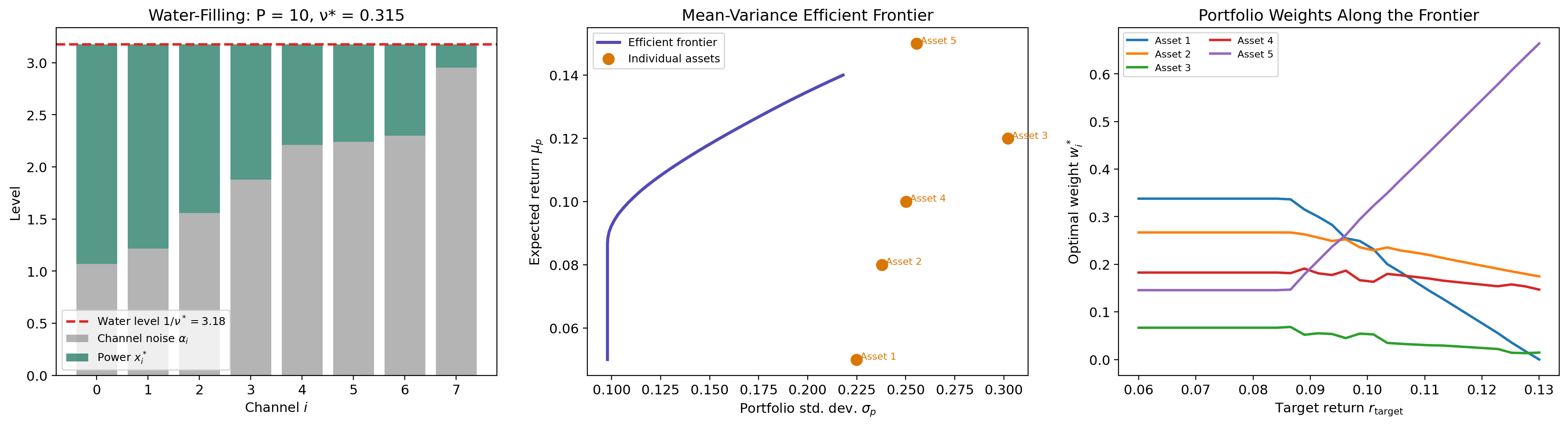
Water-Filling for Channel Capacity
In information theory, the water-filling problem allocates power across parallel channels to maximize total capacity:
where is the noise level of channel , is the power allocated to channel , and is the total power budget.
Remark (Water-Filling as KKT in Closed Form).
Writing the KKT stationarity condition for the Lagrangian and applying complementary slackness (), we get the water-filling solution:
The dual variable (the “water level”) is determined by the budget constraint . The name comes from the visualization: imagine pouring water (power) over an irregular terrain (the noise levels ); the water settles to a uniform level , filling the noisiest channels last.
import numpy as np
from scipy.optimize import brentq

def water_filling(alphas, P_total):
    """Water-filling solution via bisection for the water level."""
    def budget_residual(nu_inv):
        alloc = np.maximum(0, nu_inv - alphas)
        return np.sum(alloc) - P_total

    nu_inv_star = brentq(budget_residual, max(alphas), max(alphas) + P_total + 10)
    x_star = np.maximum(0, nu_inv_star - alphas)
    return x_star, 1.0 / nu_inv_star
Mean-Variance Portfolio Optimization
In Markowitz portfolio theory, we trace the efficient frontier by solving a family of constrained problems:
where is the return covariance matrix, is the expected return vector, and is the minimum acceptable return. The dual variable for the return constraint is the risk-return tradeoff price: it tells you how much additional variance you must accept per unit of additional expected return.
By varying from the minimum-variance portfolio to the maximum-return portfolio and solving the KKT conditions at each point, we trace the efficient frontier — the Pareto-optimal set of portfolios. The shadow price is the slope of the efficient frontier at each point.
Computational Notes
CVXPY with Automatic Dual Extraction
CVXPY is a Python-embedded modeling language for disciplined convex programming. It automatically solves the dual alongside the primal and exposes the dual variables directly.
import cvxpy as cp

x = cp.Variable(2)
objective = cp.Minimize((x[0] - 3)**2 + (x[1] - 2)**2)
constraints = [
    x[0] + x[1] <= 3,     # Resource constraint
    x[0] >= 0, x[1] >= 0  # Non-negativity
]
prob = cp.Problem(objective, constraints)
prob.solve()

print(f"Optimal value: {prob.value:.4f}")
print(f"Optimal x: {x.value}")
for i, c in enumerate(constraints):
    print(f"Constraint {i} dual value (shadow price): {c.dual_value:.4f}")
The .dual_value attribute gives directly. This is how you extract shadow prices in practice — no manual KKT derivation needed.
scipy.optimize with SLSQP
For problems not in disciplined convex form, scipy.optimize.minimize with method='SLSQP' handles nonlinear constraints:
from scipy.optimize import minimize
result = minimize(
fun=lambda x: (x[0] - 3)**2 + (x[1] - 2)**2,
x0=[0.0, 0.0],
method='SLSQP',
constraints=[
{'type': 'ineq', 'fun': lambda x: 3 - x[0] - x[1]}, # x0 + x1 <= 3
],
bounds=[(0, None), (0, None)]
)
print(f"Optimal value: {result.fun:.6f}")
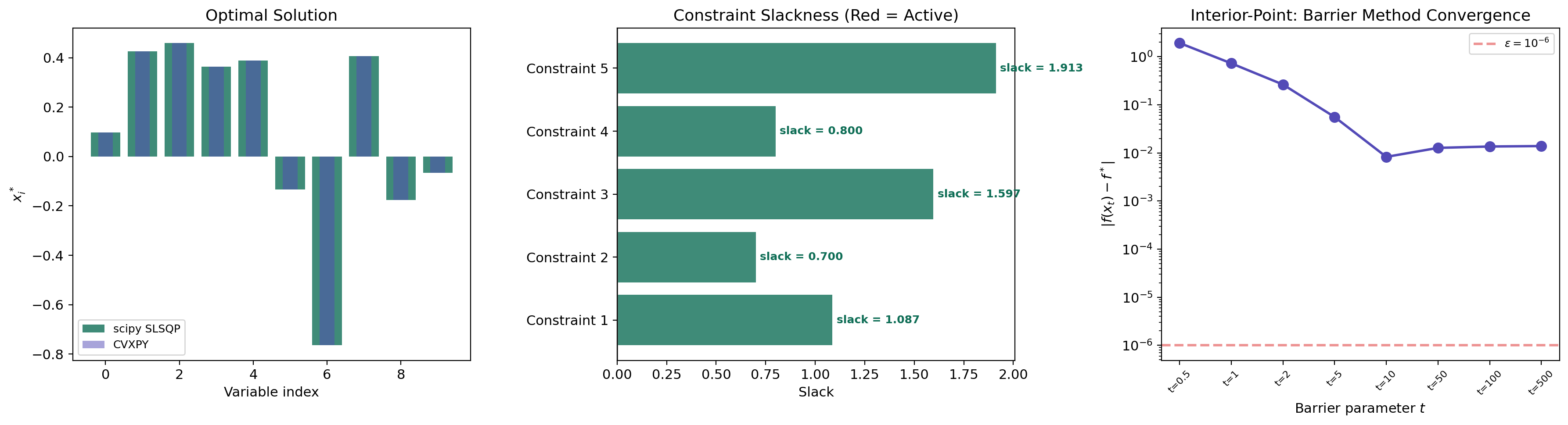
print(f"Optimal x: {result.x}")Interior-Point / Barrier Methods
Interior-point methods approach the constrained optimum from the interior of the feasible set by adding a logarithmic barrier that blows up at the constraint boundary:
As the barrier parameter , the solution traces the central path toward the true constrained optimum. At each point on the central path, the barrier Hessian system is a perturbed KKT system — interior-point methods are solving KKT conditions with a controlled perturbation. The convergence rate is typically Newton steps, where is the number of constraints.
def barrier_method(f0, grad_f0, constraints, x0, t_init=1, mu=10, tol=1e-8):
    """Conceptual barrier method — solve a sequence of unconstrained problems."""
    x = x0.copy()
    t = t_init
    while True:
        # Phase 1: centering — minimize t*f0(x) + barrier using Newton's method
        for _ in range(100):  # Inner Newton iterations
            barrier_grad = sum(-1.0 / c['fun'](x) * c['grad'](x) for c in constraints)
            total_grad = t * grad_f0(x) + barrier_grad
            x = x - 0.01 * total_grad  # Simplified: use Newton step in practice

        # Phase 2: increase t
        if len(constraints) / t < tol:
            break
        t *= mu

    return x
Constraint diagnostics. After solving, verify the KKT conditions numerically:
- Stationarity residual: should be near zero.
- Complementary slackness: should be near zero for each .
- Primal feasibility: should be (within tolerance).
- Dual feasibility: should be .
Connections & Further Reading
Lagrangian duality is the theoretical core of constrained optimization, connecting the convex analysis foundations to the algorithmic methods in the rest of the Optimization track and beyond.
| Topic | Connection |
|---|---|
| Convex Analysis | Every result here rests on convex analysis. Weak duality follows from the infimum structure; strong duality uses the separating hyperplane theorem; KKT stationarity extends the subdifferential condition to constrained settings. Conjugate functions are the engine of Lagrangian duality: the dual function for linear constraints. |
| Gradient Descent & Convergence | Interior-point methods solve the KKT system via Newton’s method on the barrier-perturbed equations. The convergence analysis of these solvers relies on the smoothness and strong convexity framework. The barrier parameter controls the tradeoff between centering accuracy and constraint satisfaction. |
| Proximal Methods | ADMM is a dual decomposition method: it applies Douglas–Rachford splitting to the dual of the consensus problem. The augmented Lagrangian is a proximal regularization of the standard Lagrangian, connecting the dual update to proximal point iterations. |
| The Spectral Theorem | Quadratic programs require the objective Hessian to be PSD for convexity. The eigendecomposition determines the condition number that governs interior-point convergence. For SDPs, the spectral theorem on the matrix variable provides the optimality structure. |
| Singular Value Decomposition | The SVM dual involves the Gram matrix . For kernel SVMs, the SVD of the feature matrix reveals the effective dimensionality and condition number of , governing the dual QP’s numerical behavior. |
| PCA & Low-Rank Approximation | Nuclear norm minimization subject to linear constraints is the convex relaxation of rank-constrained optimization. The dual of this problem involves the spectral norm, and the duality theory developed here establishes the tightness of the relaxation. |
| Adjunctions | Lagrangian duality is a Galois connection — an adjunction between posets. Weak duality () is the counit condition, strong duality () is when the unit and counit are isomorphisms, and the duality gap measures the obstruction. The KKT conditions characterize the fixed points of the closure operator. |
The Optimization Track (Complete)
Convex Analysis
    ├── Gradient Descent & Convergence
    │       └── Proximal Methods
    └── Lagrangian Duality & KKT (this topic)
This topic completes the Optimization track. The four topics form a coherent progression: Convex Analysis provides the mathematical foundations (convex sets, functions, subdifferentials, separation theorems), Gradient Descent develops the unconstrained optimization theory (smooth, strongly convex, accelerated), Proximal Methods extends to non-smooth and composite objectives (proximal operators, splitting, ADMM), and Lagrangian Duality addresses constrained optimization with the full KKT machinery.
Potential future directions that build on this foundation include second-order cone programming (SOCP), semidefinite programming (SDP), robust optimization, and bilevel optimization — but these are beyond the current curriculum scope.
Connections
- Every result in this topic rests on convex analysis. Weak duality follows from the infimum structure; strong duality requires Slater's condition on the feasible set; KKT stationarity is the multivariate extension of the subgradient optimality condition 0 ∈ ∂f(x*). The separating hyperplane theorem provides the geometric proof of strong duality. convex-analysis
- Quadratic programs min x^T P x + q^T x subject to linear constraints require P to be PSD for convexity. The Spectral Theorem provides the eigendecomposition that verifies positive semidefiniteness and computes the condition number relevant to interior-point solver convergence. spectral-theorem
- The SVM dual involves the Gram matrix K_{ij} = x_i^T x_j. For kernel SVMs, the SVD of the feature matrix reveals the effective dimensionality and condition number of the kernel matrix, governing the dual QP's difficulty. svd
- Semidefinite relaxations of rank-constrained problems (e.g., max-cut) produce SDP duals whose analysis relies on the duality theory developed here. The nuclear norm minimization from PCA & Low-Rank Approximation is the Lagrangian dual of a rank-constrained problem. pca-low-rank
- Interior-point methods solve the KKT system via Newton's method on the barrier-modified equations. The convergence analysis of these solvers uses the smoothness and strong convexity framework from the Gradient Descent topic. gradient-descent
- ADMM solves constrained problems by alternating between primal updates and dual (multiplier) updates. The augmented Lagrangian in ADMM is a proximal regularization of the standard Lagrangian developed here. proximal-methods
References & Further Reading
- book Convex Optimization — Boyd & Vandenberghe (2004) Chapter 5: Duality — the primary reference for Lagrangian duality, weak/strong duality, KKT conditions, and sensitivity analysis
- book Convex Analysis — Rockafellar (1970) The foundational monograph — conjugate duality, saddle point theory, and the minimax theorem
- book Introductory Lectures on Convex Optimization — Nesterov (2004) Chapter 4: Duality in convex optimization and self-concordant barrier methods
- book Numerical Optimization — Nocedal & Wright (2006) Chapter 12: Theory of constrained optimization — KKT conditions for general nonlinear programs
- paper A Tutorial on Support Vector Machines for Pattern Recognition — Burges (1998) The SVM dual derivation via KKT conditions and the kernel trick
- paper Interior-Point Methods in Semidefinite Programming with Applications to Combinatorial Optimization — Alizadeh (1995) Interior-point duality for SDP — extends the LP duality framework to semidefinite constraints