Proximal Methods

Overview & Motivation

In Gradient Descent & Convergence we built a complete convergence theory for smooth optimization: given an $L$-smooth convex function $f$, gradient descent with step size $\eta = 1/L$ achieves an $O(1/k)$ rate, and Nesterov acceleration pushes this to the optimal $O(1/k^2)$. But smoothness is a luxury that many real problems don’t enjoy.

Consider the Lasso — the workhorse of sparse regression:

$\min_{x} \frac{1}{2}\|Ax - b\|^2 + \lambda\|x\|_1$

The first term is smooth (its gradient is $A^\top(Ax - b)$), but the $\ell_1$ penalty $\lambda\|x\|_1$ is not differentiable at zero, which is precisely where sparsity lives. We can’t just compute $\nabla f(x_k)$ and step in the negative gradient direction, because $\nabla f$ doesn’t exist everywhere.

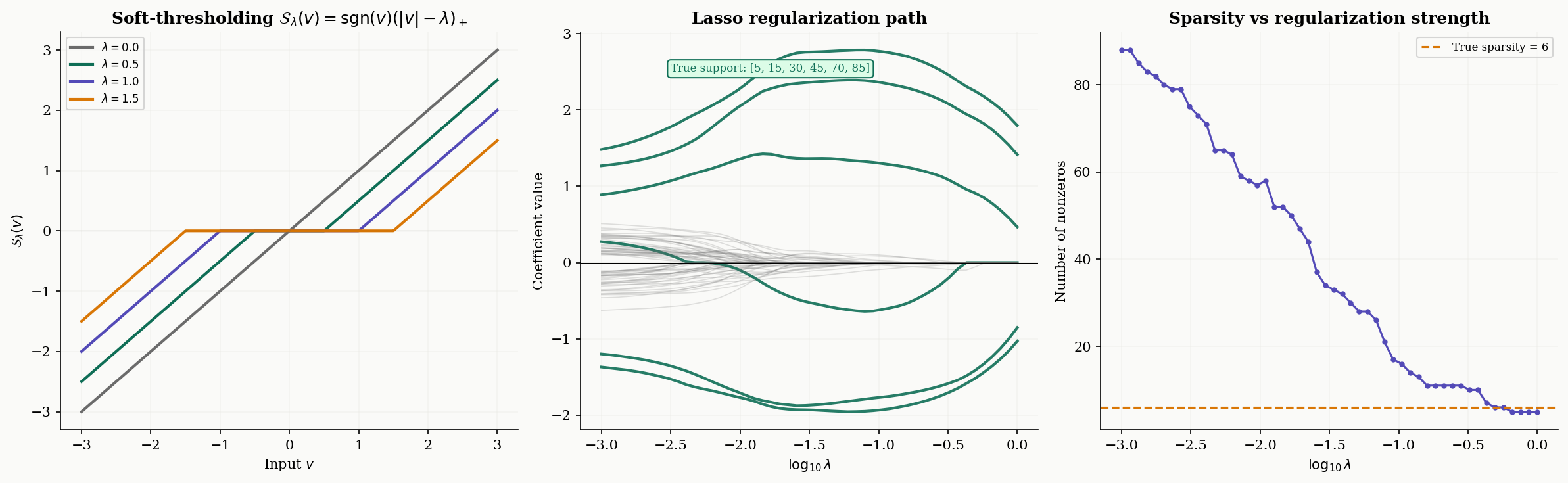
Proximal methods resolve this tension by splitting the problem into pieces we know how to handle. The key insight: even though $\|x\|_1$ isn’t smooth, we can evaluate its proximal operator — a generalization of the gradient step that replaces “move in the direction that decreases $f$ fastest” with “find the point that best balances minimizing $f$ and staying close to where you are.” For the $\ell_1$ norm, this proximal operator turns out to be soft-thresholding: shrink each coordinate toward zero by $\lambda$, and set it exactly to zero if it’s smaller than $\lambda$.

What We Cover

1. The Proximal Operator — definition, geometric interpretation, and the fixed-point characterization of minimizers.
2. Proximal Operator Catalog — closed-form solutions for the $\ell_1$ norm (soft-thresholding), indicator functions (projection), the squared norm (shrinkage), and group norms.
3. The Moreau Envelope — the smooth approximation that connects proximal operators to gradient-based reasoning, with the gradient identity $\nabla M_\lambda f = \frac{1}{\lambda}(v - \mathrm{prox}_{\lambda f}(v))$.
4. Proximal Gradient Descent — forward-backward splitting for composite objectives $F = g + h$ (smooth + non-smooth), with $O(1/k)$ convergence.
5. ISTA — proximal gradient applied to the Lasso, with soft-thresholding as the key subroutine.
6. FISTA — Nesterov-style acceleration from $O(1/k)$ to the optimal $O(1/k^2)$.
7. Douglas–Rachford Splitting — handling problems where both terms are non-smooth.
8. ADMM — the consensus formulation with three-variable updates and primal-dual residuals.
9. Convergence Analysis — the rate landscape across algorithms and the role of strong convexity.
10. Computational Notes — backtracking step size selection, convergence diagnostics, and stopping criteria.

---

The Proximal Operator

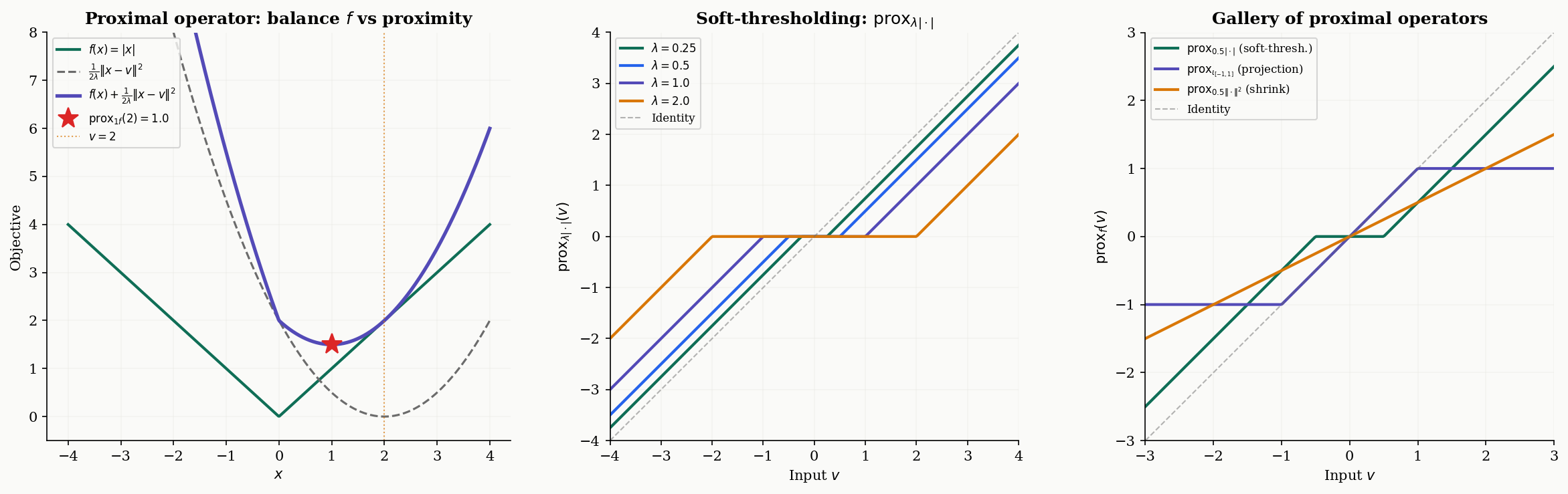
The proximal operator is the fundamental building block. Where gradient descent asks “which direction decreases $f$ fastest?”, the proximal operator asks a different question: “which point best balances minimizing $f$ and staying close to where I am?”

The parameter $\lambda$ controls the tradeoff between the two competing objectives. When $\lambda$ is small, the quadratic penalty dominates — the proximal operator stays close to $v$, barely moving. When $\lambda$ is large, the function $f$ dominates — the proximal operator moves toward the minimizer of $f$ itself. In the limit $\lambda \to 0$, $\mathrm{prox}_{\lambda f}(v) \to v$ (don’t move); in the limit $\lambda \to \infty$, $\mathrm{prox}_{\lambda f}(v) \to \arg\min f$ (jump to the global minimizer).

The proximal operator has an elegant characterization in terms of fixed points that connects it directly to the optimality conditions from Convex Analysis.

λ1.0|x| (soft-thresholding)ι_{[-1,1]} (projection)x² (shrinkage)|x| + ι_{[0,∞)} (non-neg soft-thresh)

prox_λf(v) = prox_1.0·|x|(1.5) = 0.500

---

Proximal Operator Catalog

The utility of proximal methods depends on having cheap, closed-form proximal operators for the functions we care about. Here are the most important ones.

Soft-thresholding is the engine behind every $\ell_1$-regularized method in this topic. It does two things simultaneously: it shrinks each coordinate toward zero by $\lambda$ (the “shrinkage” part), and it sets coordinates smaller than $\lambda$ exactly to zero (the “thresholding” part). This is why $\ell_1$ regularization produces sparse solutions — the proximal operator itself enforces sparsity.

def soft_threshold(x, lam):
    """Proximal operator of lambda * |.|: soft-thresholding."""
    return np.sign(x) * np.maximum(np.abs(x) - lam, 0.0)

This is immediate from the definition: the term $\iota_C(x)$ forces the minimizer to lie in $C$, and the quadratic penalty selects the closest point in $C$ to $v$. The indicator function effectively encodes a hard constraint, and its proximal operator is the classical projection. This means constrained optimization can be cast as unconstrained proximal operations.

This follows by setting the gradient of $\frac{1}{2}\|x\|^2 + \frac{1}{2\lambda}\|x - v\|^2$ to zero: $(1 + 1/\lambda)x = v/\lambda$, giving $x = v/(1 + \lambda)$.

Two more proximal operators appear frequently in applications:

Group soft-thresholding. For the group Lasso with $f(x) = \|x_G\|_2$ (the $\ell_2$ norm of a group of coordinates), the proximal operator is:

$\mathrm{prox}_{\lambda f}(v_G) = \begin{cases} \left(1 - \frac{\lambda}{\|v_G\|_2}\right) v_G & \text{if } \|v_G\|_2 > \lambda \\ 0 & \text{otherwise} \end{cases}$

This zeroes out entire groups, rather than individual coordinates.

Simplex projection. The proximal operator of the indicator of the probability simplex $\Delta = \{x \geq 0 : \sum_i x_i = 1\}$ is the Euclidean projection onto $\Delta$. This can be computed in $O(n \log n)$ time by sorting and thresholding (Duchi et al., 2008):

def proj_simplex(x):
    """Projection onto the probability simplex."""
    n = len(x)
    u = np.sort(x)[::-1]
    cssv = np.cumsum(u) - 1.0
    rho = np.nonzero(u * np.arange(1, n + 1) > cssv)[0][-1]
    theta = cssv[rho] / (rho + 1.0)
    return np.maximum(x - theta, 0.0)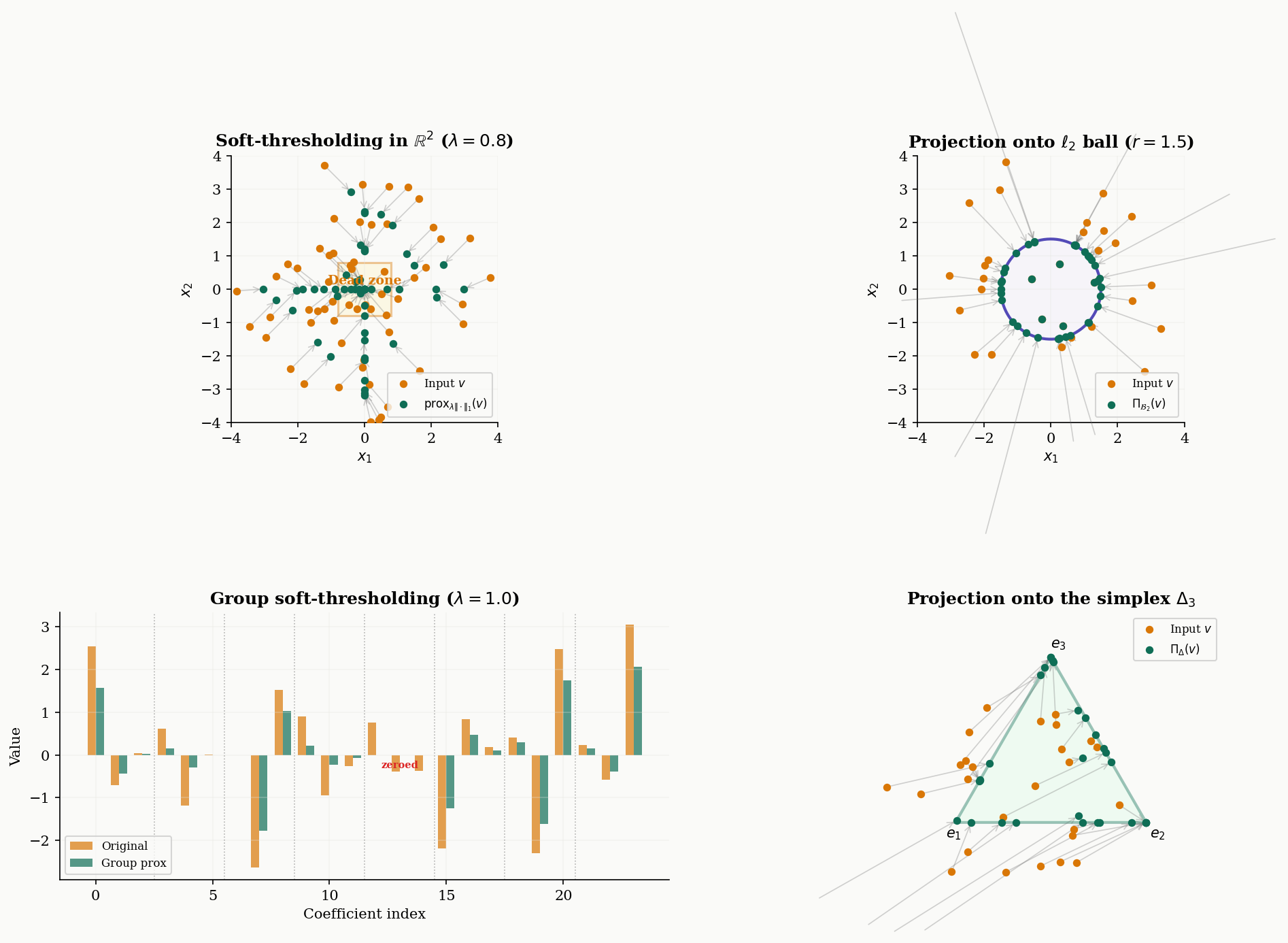

---

The Moreau Envelope

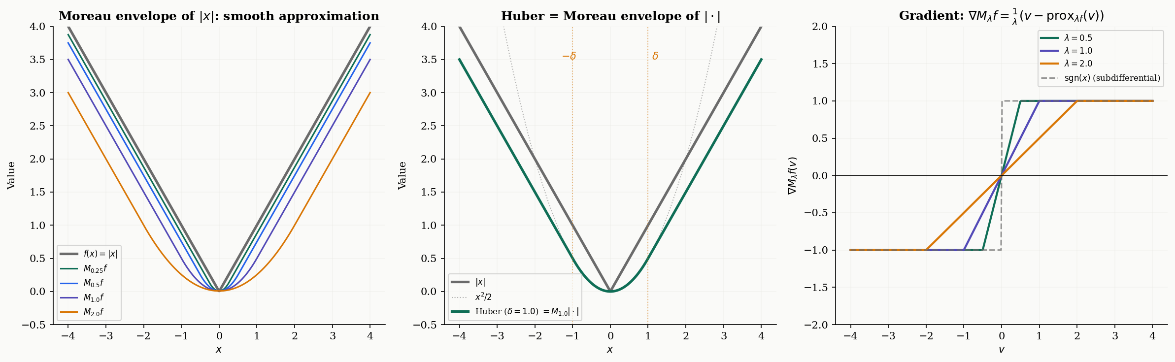
The proximal operator finds the minimizer of $f(x) + \frac{1}{2\lambda}\|x - v\|^2$. But what is the value of that minimum? This is the Moreau envelope — a smooth version of $f$ that serves as a theoretical bridge between non-smooth analysis and gradient-based reasoning.

The parameter $\lambda$ controls the smoothing strength. When $\lambda$ is small, $M_\lambda f$ closely approximates $f$ (but with corners rounded off). When $\lambda$ is large, $M_\lambda f$ is a very smooth, gentle version of $f$. The infimal values are preserved: $\min M_\lambda f = \min f$, and the minimizers are the same.

A beautiful special case: when $f(x) = |x|$, the Moreau envelope $M_\lambda |{\cdot}|$ is exactly the Huber function with parameter $\delta = \lambda$:

$M_\lambda |\cdot|(v) = \begin{cases} \frac{v^2}{2\lambda} & \text{if } |v| \leq \lambda \\ |v| - \frac{\lambda}{2} & \text{if } |v| > \lambda \end{cases}$

The Huber function is the standard “smooth $\ell_1$” used in robust regression — it’s quadratic near zero and linear in the tails, and we now see that this arises naturally as the Moreau envelope.

This identity is remarkable: the gradient of the smooth envelope equals the proximal residual $\frac{1}{\lambda}(v - \mathrm{prox}_{\lambda f}(v))$, scaled by $1/\lambda$. When $v = x^*$ is a minimizer, the proximal operator is the identity ($x^* = \mathrm{prox}_{\lambda f}(x^*)$), and the gradient is zero — exactly what we expect.

---

Proximal Gradient Descent

Now we assemble the proximal operator into an optimization algorithm. The setting is composite minimization — the most important problem structure in modern convex optimization.

The canonical example is the Lasso: $g(x) = \frac{1}{2}\|Ax - b\|^2$ is smooth with $L = \lambda_{\max}(A^\top A)$, and $h(x) = \lambda\|x\|_1$ has the soft-thresholding proximal operator. But the framework covers much more — any problem where we can split the objective into a smooth part we can take gradients of and a structured part we can “prox.”

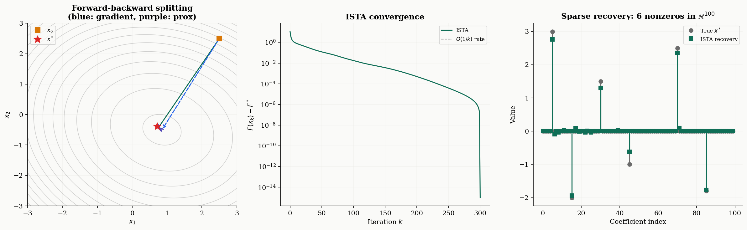
The forward-backward splitting algorithm alternates between a gradient step on $g$ (the “forward” step) and a proximal step on $h$ (the “backward” step):

$x_{k+1} = \mathrm{prox}_{\eta h}\!\left(x_k - \eta \nabla g(x_k)\right)$

where $\eta \in (0, 1/L]$ is the step size. Intuitively: first move in the negative gradient direction of $g$ (the smooth part), then apply the proximal operator of $h$ to “clean up” — projecting, thresholding, or whatever $h$ demands.

When $h = 0$, the proximal step is the identity and we recover vanilla gradient descent. When $g = 0$, the gradient step is trivial and we get the proximal point algorithm. Forward-backward splitting is the natural hybrid.

---

ISTA & Soft-Thresholding

The Iterative Shrinkage-Thresholding Algorithm (ISTA) is proximal gradient descent applied to the Lasso. The name comes from the fact that the proximal step reduces to componentwise soft-thresholding — a “shrink and threshold” operation.

The two-step structure is transparent. The gradient step $x_k - \eta A^\top(Ax_k - b)$ moves toward fitting the data (minimizing $\|Ax - b\|^2$), and the soft-thresholding step $\mathcal{S}_{\eta\lambda}$ promotes sparsity by shrinking small coefficients to zero. The threshold $\eta\lambda$ balances the two goals: larger $\lambda$ means more thresholding and sparser solutions.

# ISTA for Lasso
L = np.linalg.eigvalsh(A.T @ A)[-1]  # Lipschitz constant
eta = 1.0 / L
x = np.zeros(p)

for k in range(max_iter):
    x_half = x - eta * A.T @ (A @ x - b)          # gradient step on g
    x = soft_threshold(x_half, eta * lam_lasso)     # prox step on h

The regularization path. As $\lambda$ varies from large to small, the ISTA solution traces a path from zero (complete sparsity) to the least-squares solution (no regularization). This path reveals which features enter the model first — the most important predictors appear at larger $\lambda$ values. Computing the full regularization path is a standard diagnostic for choosing $\lambda$ in practice.

---

FISTA: Accelerated Proximal Gradient

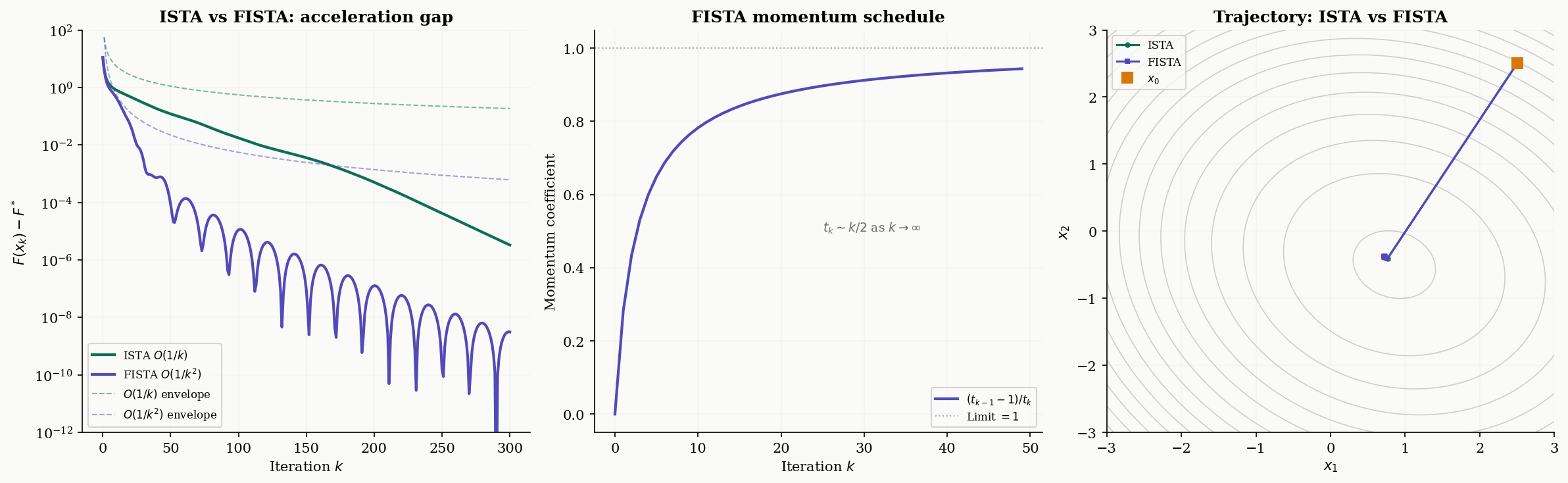
ISTA’s $O(1/k)$ rate is the same as vanilla gradient descent on smooth problems. Can we accelerate it, the way Nesterov acceleration improves gradient descent from $O(1/k)$ to $O(1/k^2)$? The answer is yes, and the result is FISTA — the Fast Iterative Shrinkage-Thresholding Algorithm of Beck & Teboulle (2009).

The momentum schedule $t_{k+1} = \frac{1 + \sqrt{1 + 4t_k^2}}{2}$ is the signature feature. As $k \to \infty$, the momentum coefficient $(t_{k-1} - 1)/t_k \to 1$, meaning the extrapolation step becomes increasingly aggressive. This is why FISTA trajectories can overshoot — the momentum pushes past the current iterate, trading local stability for faster global convergence.

# FISTA for Lasso
x = np.zeros(p)
x_prev = x.copy()
t_k = 1.0

for k in range(max_iter):
    t_next = (1 + np.sqrt(1 + 4 * t_k**2)) / 2
    y = x + ((t_k - 1) / t_next) * (x - x_prev)   # momentum extrapolation
    x_prev = x.copy()
    x_half = y - eta * A.T @ (A @ y - b)            # gradient step on g (at y)
    x = soft_threshold(x_half, eta * lam_lasso)      # prox step on h
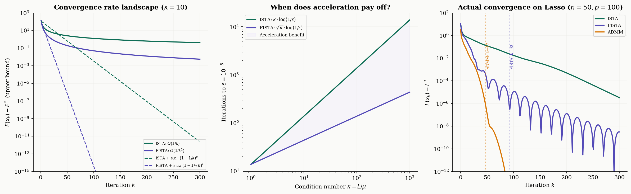
    t_k = t_next

When does acceleration matter? The gap between $O(1/k)$ and $O(1/k^2)$ is most dramatic when high accuracy is needed — to reach $\epsilon = 10^{-6}$, ISTA needs $O(1/\epsilon)$ iterations while FISTA needs $O(1/\sqrt{\epsilon})$. For well-conditioned problems or moderate accuracy, ISTA may suffice. For ill-conditioned sparse recovery or high-precision scientific computing, FISTA’s speedup is substantial.

κ10Show momentum

---

Douglas–Rachford Splitting

Forward-backward splitting requires one term to be smooth (so we can compute its gradient). What if both terms are non-smooth? This is the setting for Douglas–Rachford splitting.

The variable $z_k$ is an auxiliary “shadow” variable — it doesn’t converge to the solution itself, but the $y_k$ iterates do. The second update can be rewritten as $z_{k+1} = z_k + R_g \circ R_f(z_k)$ where $R_f(z) = 2\mathrm{prox}_f(z) - z$ is the reflected proximal operator (or “reflection”). Douglas–Rachford is thus an averaged iteration of composed reflections — a deeply geometric operation.

The canonical application is basis pursuit: minimize $\|x\|_1$ subject to $Ax = b$ (exact sparse recovery). Setting $f(x) = \|x\|_1$ and $g(x) = \iota_{\{Ax = b\}}(x)$, both are non-smooth, but both have cheap proximal operators — soft-thresholding for $f$ and projection onto the affine subspace for $g$.

# Douglas-Rachford for basis pursuit: min ||x||_1 s.t. Ax = b
AAt_inv = np.linalg.inv(A @ A.T)
def proj_affine(x):
    return x + A.T @ AAt_inv @ (b - A @ x)

gamma = 1.0
z = np.zeros(p)
for k in range(max_iter):
    y = soft_threshold(z, gamma)                    # prox_f
    r = proj_affine(2 * y - z)                      # prox_g(reflected)
    z = z + r - y                                   # shadow update
# y is the solution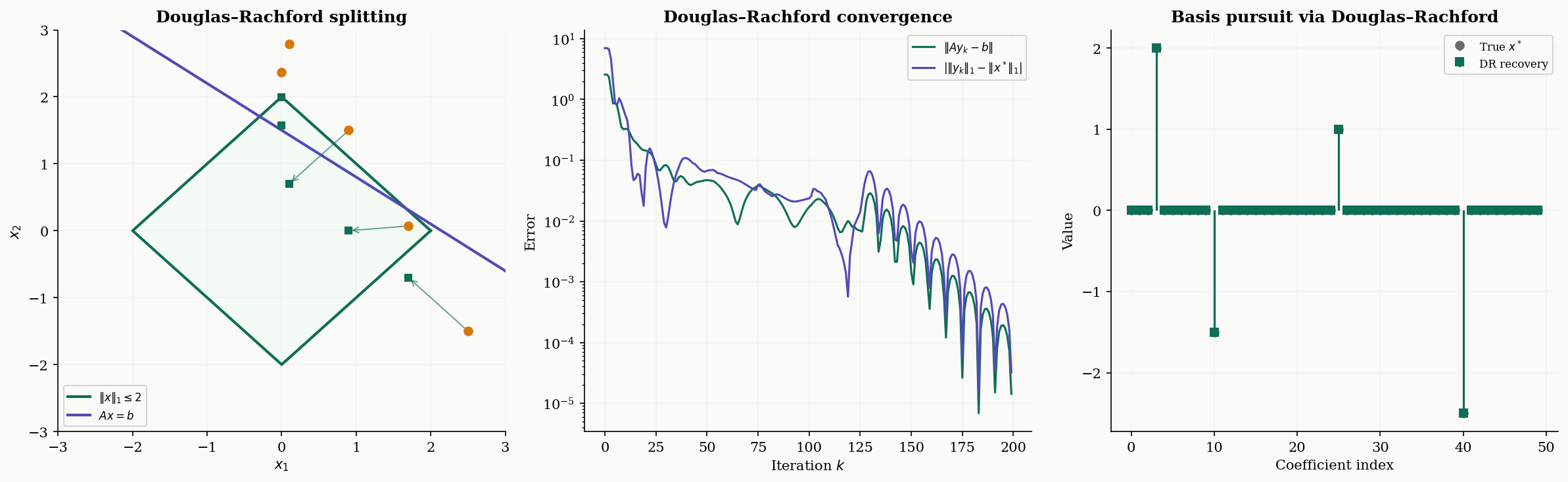

---

ADMM

The Alternating Direction Method of Multipliers (ADMM) is the most widely used splitting method in practice. It handles the general constrained formulation $\min f(x) + g(z) \text{ s.t. } Ax + Bz = c$ by augmenting the Lagrangian with a quadratic penalty.

For the Lasso via ADMM, we set $f(x) = \frac{1}{2}\|Ax - b\|^2$ and $g(z) = \lambda\|z\|_1$ with the constraint $x = z$. The $x$-update requires solving a linear system $(A^\top A + \rho I)x = A^\top b + \rho(z - u)$, the $z$-update is soft-thresholding, and the $u$-update is a simple addition.

# ADMM for Lasso
rho = 1.0
AtA_rho_inv = np.linalg.inv(A.T @ A + rho * np.eye(p))
Atb = A.T @ b

x, z, u = np.zeros(p), np.zeros(p), np.zeros(p)
for k in range(max_iter):
    x = AtA_rho_inv @ (Atb + rho * (z - u))              # x-update
    z_old = z.copy()
    z = soft_threshold(x + u, lam_lasso / rho)            # z-update
    u = u + x - z                                          # dual update

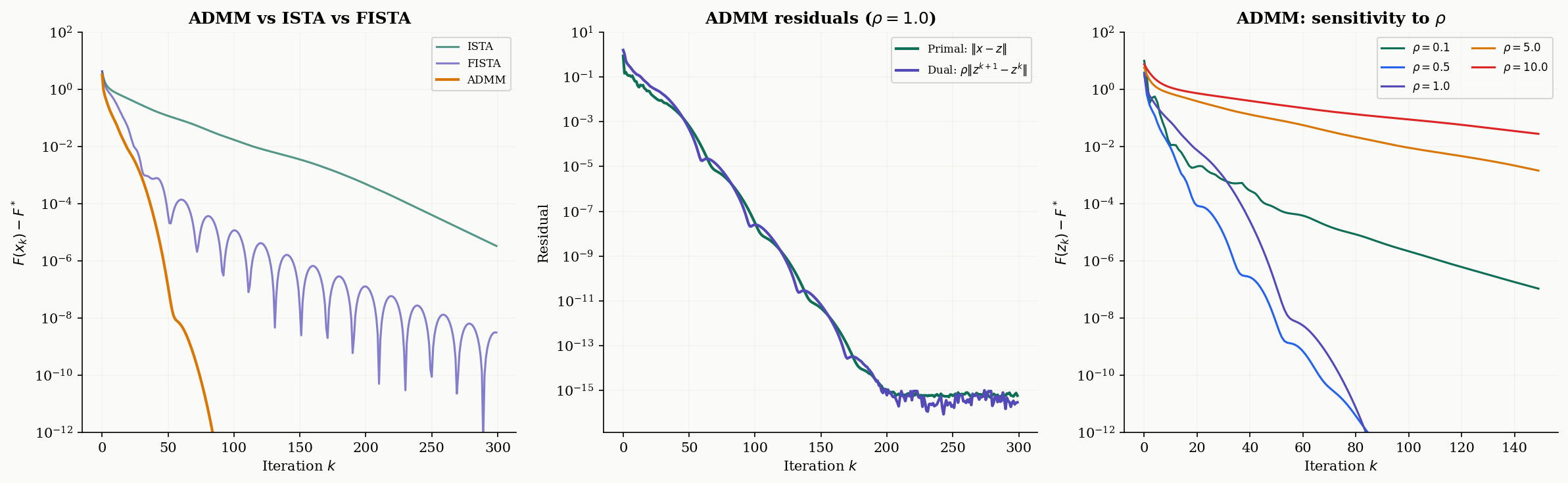
    primal_res = np.linalg.norm(x - z)                    # primal residual
    dual_res = rho * np.linalg.norm(z - z_old)            # dual residual

Convergence monitoring. ADMM convergence is tracked via two residuals:

• Primal residual $r_k = \|x_k - z_k\|$ — measures constraint violation (how far $x$ and $z$ are from consensus).
• Dual residual $s_k = \rho\|z_k - z_{k-1}\|$ — measures dual variable change (stationarity of the Lagrangian).

The algorithm converges when both residuals are small. The standard stopping criterion is $r_k < \epsilon^{\mathrm{pri}}$ and $s_k < \epsilon^{\mathrm{dual}}$.

Sensitivity to $\rho$. The penalty parameter $\rho$ has a significant effect on convergence speed but does not affect the final solution. Small $\rho$ favors fast primal convergence (the $x$ and $z$ updates are more independent), while large $\rho$ favors fast dual convergence (the constraint is enforced more aggressively). In practice, adaptive $\rho$ schemes that increase $\rho$ when the primal residual is large and decrease it when the dual residual is large can dramatically improve convergence.

ρ1.00Show residualsADMM onlyADMM vs ISTA vs FISTA

---

Convergence Analysis

We now have four splitting algorithms — ISTA, FISTA, Douglas–Rachford, and ADMM — each designed for a different problem structure. The following table summarizes the convergence landscape:

Algorithm	Setting	Rate (convex)	Rate (strongly convex, $\mu > 0$)
ISTA (Proximal Gradient)	$g$ smooth + $h$ prox-friendly	$O(LR^2/k)$	$(1 - \mu/L)^k$ (linear)
FISTA (Accelerated)	$g$ smooth + $h$ prox-friendly	$O(LR^2/k^2)$ (optimal)	$(1 - \sqrt{\mu/L})^k$ (linear, faster)
Douglas–Rachford	both non-smooth, both prox-friendly	$O(1/k)$	—
ADMM	consensus/splitting form	$O(1/k)$	—

Here $L$ is the smoothness constant of $g$, $R = \|x_0 - x^*\|$ is the initial distance, $\mu$ is the strong convexity parameter, and $\kappa = L/\mu$ is the condition number.

Key observations:

1. FISTA is always at least as fast as ISTA, and strictly faster when the target accuracy $\epsilon$ is small. The gap widens as $\kappa$ grows: ISTA needs $O(\kappa \log(1/\epsilon))$ iterations while FISTA needs $O(\sqrt{\kappa}\log(1/\epsilon))$.

2. Strong convexity accelerates both ISTA and FISTA from sublinear to linear convergence. The practical message: if you know your problem is strongly convex, the convergence is exponentially faster.

3. ADMM and DR have the same theoretical rate ($O(1/k)$), but ADMM is often faster in practice because it exploits the structure of the consensus formulation and allows per-variable parallelism.

4. Condition number dependence is the bottleneck. For all these methods, ill-conditioned problems (large $\kappa$) converge slowly. Preconditioning — transforming the problem to reduce $\kappa$ — is often more effective than switching algorithms.

---

Computational Notes

We close with a full implementation of proximal gradient descent with Armijo backtracking — the version you’d actually use in practice, with convergence diagnostics.

Backtracking step size selection. Instead of computing $L = \lambda_{\max}(A^\top A)$ exactly (which requires an eigendecomposition), backtracking finds a suitable step size adaptively. Starting from an initial estimate $L_{\text{est}}$, it doubles $L_{\text{est}}$ until the sufficient decrease condition is satisfied:

$g(x_{k+1}) \leq g(y) + \langle \nabla g(y), x_{k+1} - y \rangle + \frac{L_{\text{est}}}{2}\|x_{k+1} - y\|^2$

This ensures the step size is never too large while allowing it to be larger than $1/L$ when the local curvature is smaller.

def proximal_gradient_bt(A, b, lam, x0=None, max_iter=500, tol=1e-8,
                          accelerated=False, verbose=False):
    """
    Proximal gradient for Lasso: min (1/2)||Ax-b||^2 + lam*||x||_1
    with Armijo backtracking for step size selection.

    Parameters
    ----------
    A : (n, p) array
    b : (n,) array
    lam : float, regularization parameter
    x0 : initial point (default: zeros)
    max_iter : max iterations
    tol : stopping tolerance on relative change
    accelerated : if True, use FISTA momentum

    Returns
    -------
    x : solution
    info : dict with convergence diagnostics
    """
    n_obs, p_dim = A.shape
    if x0 is None:
        x0 = np.zeros(p_dim)

    x = x0.copy()
    x_prev = x.copy()
    t_k = 1.0
    L_est = 1.0

    AtA = A.T @ A
    Atb_vec = A.T @ b

    info = {'f_vals': [], 'grad_norms': [], 'step_sizes': [], 'nnz': []}

    def f_smooth(x):
        r = A @ x - b
        return 0.5 * np.dot(r, r)

    def grad_smooth(x):
        return AtA @ x - Atb_vec

    def F_obj(x):
        return f_smooth(x) + lam * np.linalg.norm(x, 1)

    for k in range(max_iter):
        if accelerated and k > 0:
            t_next = (1 + np.sqrt(1 + 4 * t_k**2)) / 2
            y = x + ((t_k - 1) / t_next) * (x - x_prev)
            t_k = t_next
        else:
            y = x

        g = grad_smooth(y)
        f_y = f_smooth(y)

        # Backtracking: find step size that satisfies descent condition
        while True:
            eta_k = 1.0 / L_est
            x_new = soft_threshold(y - eta_k * g, eta_k * lam)
            f_new = f_smooth(x_new)
            d = x_new - y
            if f_new <= f_y + np.dot(g, d) + (L_est / 2) * np.dot(d, d):
                break
            L_est *= 2

        # Adaptive decrease of L_est for efficiency
        if k % 10 == 0 and L_est > 1.0:
            L_est *= 0.8

        x_prev = x.copy()
        x = x_new

        info['f_vals'].append(F_obj(x))
        info['grad_norms'].append(np.linalg.norm(g))
        info['step_sizes'].append(eta_k)
        info['nnz'].append(np.sum(np.abs(x) > 1e-8))

        # Stopping criterion: relative change
        if k > 0 and abs(info['f_vals'][-1] - info['f_vals'][-2]) < tol * abs(info['f_vals'][-2]):
            break

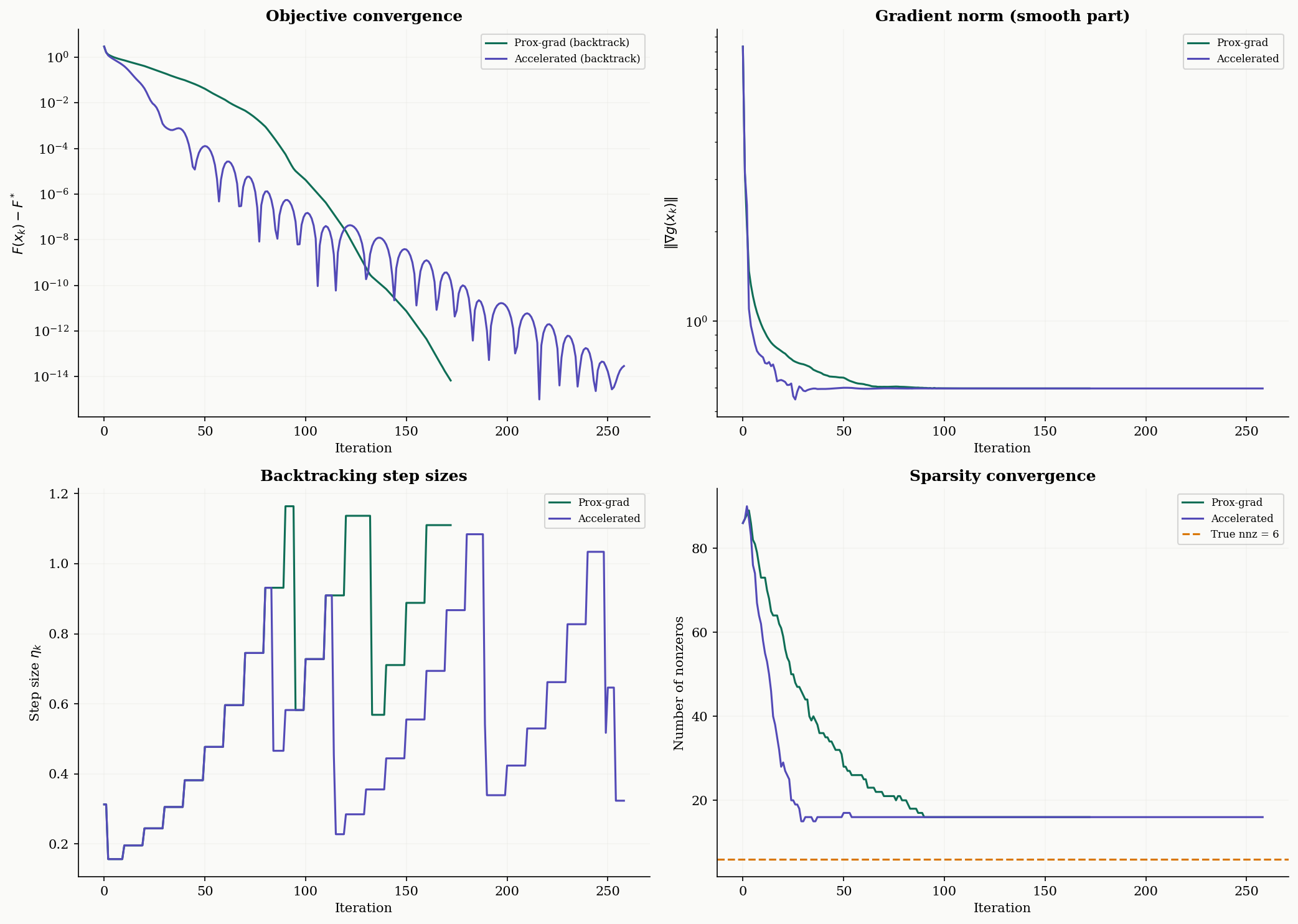
    return x, info

Convergence diagnostics. A well-implemented proximal gradient solver tracks four quantities:

1. Objective value $F(x_k)$ — should decrease monotonically (for ISTA; FISTA may oscillate).
2. Gradient norm $\|\nabla g(x_k)\|$ — measures how close the smooth part is to stationarity.
3. Step size $\eta_k$ — should stabilize; rapid changes indicate numerical issues.
4. Sparsity $\|x_k\|_0$ (number of nonzeros) — should converge to a stable support.

---

Connections & Further Reading

Proximal methods sit at the intersection of convex analysis, gradient-based optimization, and linear algebra — drawing on the foundations of the first two topics in the Optimization track and connecting forward to constrained optimization.

Topic	Connection
Convex Analysis	Every proximal operator solves a convex minimization problem. The subdifferential optimality condition $0 \in \partial f(x^*)$ becomes the fixed-point condition $x^* = \mathrm{prox}_f(x^*)$. Conjugate functions and the Moreau envelope are dual objects connected by the Fenchel–Moreau theorem.
Gradient Descent & Convergence	Proximal gradient descent generalizes gradient descent to composite objectives $F = g + h$. When $h = 0$, the proximal step reduces to the identity and we recover vanilla GD. The convergence analysis parallels the Descent Lemma, and FISTA inherits Nesterov’s momentum machinery. Mirror descent from GD is a special case of the proximal point algorithm with Bregman divergence.
The Spectral Theorem	The condition number $\kappa = L/\mu$ that governs proximal gradient convergence involves eigenvalues of the Hessian. For quadratic $g(x) = \frac{1}{2}x^\top A x$, the Spectral Theorem gives the eigendecomposition that determines $L$ and $\mu$.
Singular Value Decomposition	The proximal operator of the nuclear norm $\|X\|_* = \sum \sigma_i$ requires computing the SVD and applying soft-thresholding to the singular values — the singular value thresholding operator, which is the key subroutine in low-rank matrix recovery.
Lagrangian Duality & KKT	ADMM is a dual decomposition method: it applies Douglas–Rachford to the dual of the consensus problem. The KKT conditions generalize the fixed-point characterization $0 \in \partial f(x^*)$ to constrained settings.

The Optimization Track

Convex Analysis
    ├── Gradient Descent & Convergence
    │       └── Proximal Methods (this topic)
    └── Lagrangian Duality & KKT