Minimum Description Length

Overview & Motivation

Every statistician and every machine learning practitioner faces the same core problem: given data, which model should we use? Fit a polynomial of degree 3 or degree 15? Use a Gaussian mixture with 2 components or 20? The model that fits the training data best — the one with the highest likelihood — is almost never the right answer, because it overfits. We need a principled way to balance fit against complexity.

The Minimum Description Length (MDL) principle, introduced by Jorma Rissanen in 1978, provides exactly that balance by reframing model selection as a compression problem. The idea is beautifully concrete: imagine you want to send your dataset to a colleague using as few bits as possible. You can first describe a model (costing $L(M)$ bits), then describe the data given that model (costing $L(D \mid M)$ bits). The best model is the one that minimizes the total description length:

$L(M) + L(D \mid M)$

A simple model costs few bits to describe but leaves large residuals; a complex model describes the data well but costs many bits itself. The minimum is the sweet spot — the model that captures the genuine structure in the data without encoding noise.

This is Occam’s Razor made precise: among models that explain the data equally well, prefer the simplest one — and “simplest” means “shortest to describe.”

Prerequisites: This topic builds on KL Divergence & f-Divergences, particularly the information-theoretic interpretation of divergence as coding redundancy. Familiarity with Shannon Entropy & Mutual Information is essential — especially source coding and the connection between entropy and optimal code lengths.

What We Cover

Two-part codes and crude MDL — the description-length trade-off $L(M) + L(D \mid M)$ , Rissanen’s universal code for integers, and model selection as compression
Kolmogorov complexity — the ideal but uncomputable measure of descriptive complexity, and why MDL provides a practical alternative
Stochastic complexity and refined MDL — the Normalized Maximum Likelihood distribution, parametric complexity, and Shtarkov’s minimax optimality theorem
Fisher information and asymptotic complexity — the geometric structure hidden inside model complexity, and why BIC is a crude MDL approximation
MDL and Bayesian model selection — the surprising asymptotic equivalence of stochastic complexity and the marginal likelihood under Jeffreys prior
Prequential codes and online MDL — sequential model selection that avoids the normalization problem entirely
MDL for practical model selection — feature selection, distribution family selection, and overfitting detection

Two-Part Codes & Crude MDL

The simplest version of MDL works with two-part codes: first encode the model, then encode the data given the model. We need to make both parts precise.

Encoding Models

Suppose our model class is a family of polynomials of degree $d$ . To encode “degree $d$ ,” we need a code for positive integers. Using a fixed-length code wastes bits on small values; a variable-length code does better.

Definition 1 (Two-Part Code / Crude MDL).

Given a countable collection of models $\{M_1, M_2, \ldots\}$ and a coding scheme that assigns code length $L(M)$ to each model and $L(D \mid M)$ to the data given model $M$ , the crude MDL principle selects the model minimizing:

$\hat{M} = \arg\min_{M} \left[ L(M) + L(D \mid M) \right]$

where $L(D \mid M)$ is typically the negative log-likelihood under the maximum likelihood estimator:

$L(D \mid M) = -\log_2 p(x^n \mid \hat{\theta}(x^n), M)$

For the model code length, Rissanen proposed a universal code for positive integers:

Definition 2 (Universal Code for Integers).

Rissanen’s universal code assigns to positive integer $k$ the code length:

$L^*(k) = \log_2 k + \log_2 \log_2 k + \log_2 \log_2 \log_2 k + \cdots + \log_2 c_0$

where the sum includes only positive terms. The constant $c_0 \approx 2.865$ normalizes the code so that the implied distribution $2^{-L^*(k)}$ sums to 1 over positive integers. This is a universal code: it does not assume any prior distribution on model complexity.

Example: Polynomial Regression

Consider fitting a polynomial of degree $d$ to $n$ noisy observations. The model $M_d$ has $d + 1$ free parameters (coefficients). Using $b$ bits of precision per coefficient, the two-part code length is:

$L(M_d) + L(D \mid M_d) = \underbrace{L^*(d+1) + (d+1) \cdot b}_{\text{model complexity}} + \underbrace{\frac{n}{2} \log_2(2\pi e \hat{\sigma}^2)}_{\text{data fit}}$

where $\hat{\sigma}^2 = \text{RSS}/n$ is the residual variance under the degree- $d$ fit. The model code grows with $d$ ; the data code shrinks as the fit improves. The minimum total code length selects a degree that balances these competing pressures.

The interactive visualization below demonstrates this trade-off. Try increasing the noise level — MDL selects simpler models when the signal-to-noise ratio is low.

Max degree:12Noise σ:0.30n:

Three-panel figure showing polynomial fits, two-part code decomposition, and the Occam's sweet spot

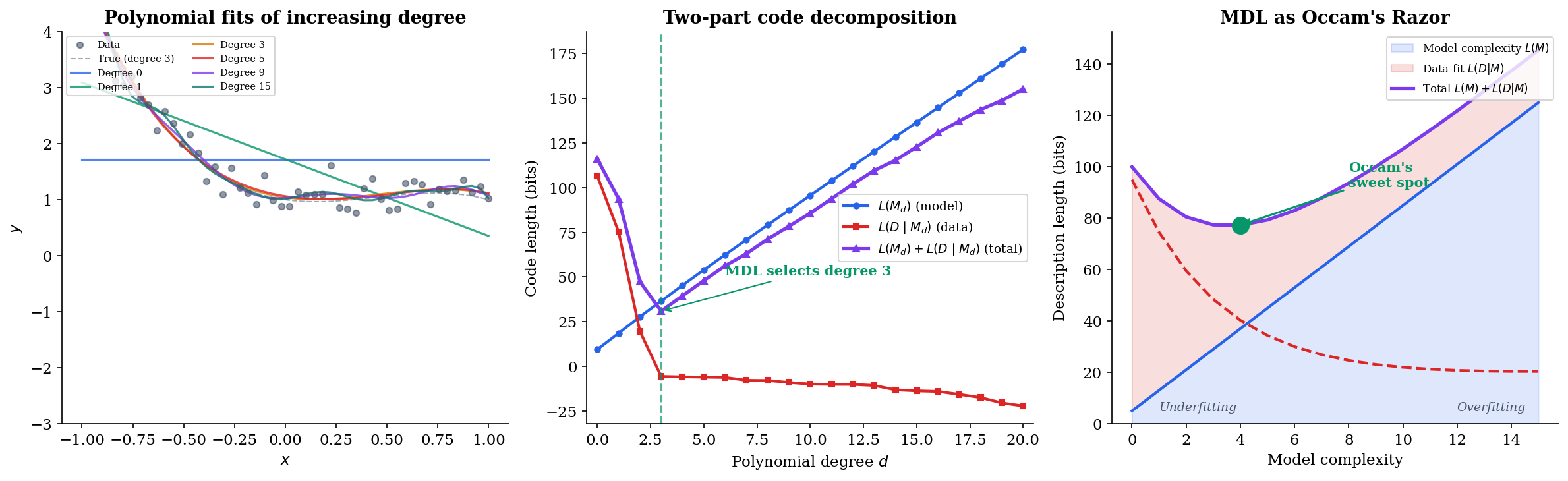
The left panel shows how the polynomial fit tightens as degree increases; the right panel reveals the two-part code decomposition. The total code length (purple line) reaches its minimum at a degree that neither underfits nor overfits — this is the MDL-optimal model.

Kolmogorov Complexity

Before we can refine MDL, we need to understand the ideal notion of descriptive complexity — one that Rissanen’s practical MDL approximates.

Definition 3 (Kolmogorov Complexity).

The Kolmogorov complexity of a binary string $x$ with respect to a universal Turing machine $U$ is:

$K_U(x) = \min \{ |p| : U(p) = x \}$

where $|p|$ denotes the length of program $p$ in bits. In words: $K_U(x)$ is the length of the shortest program that outputs $x$ and halts.

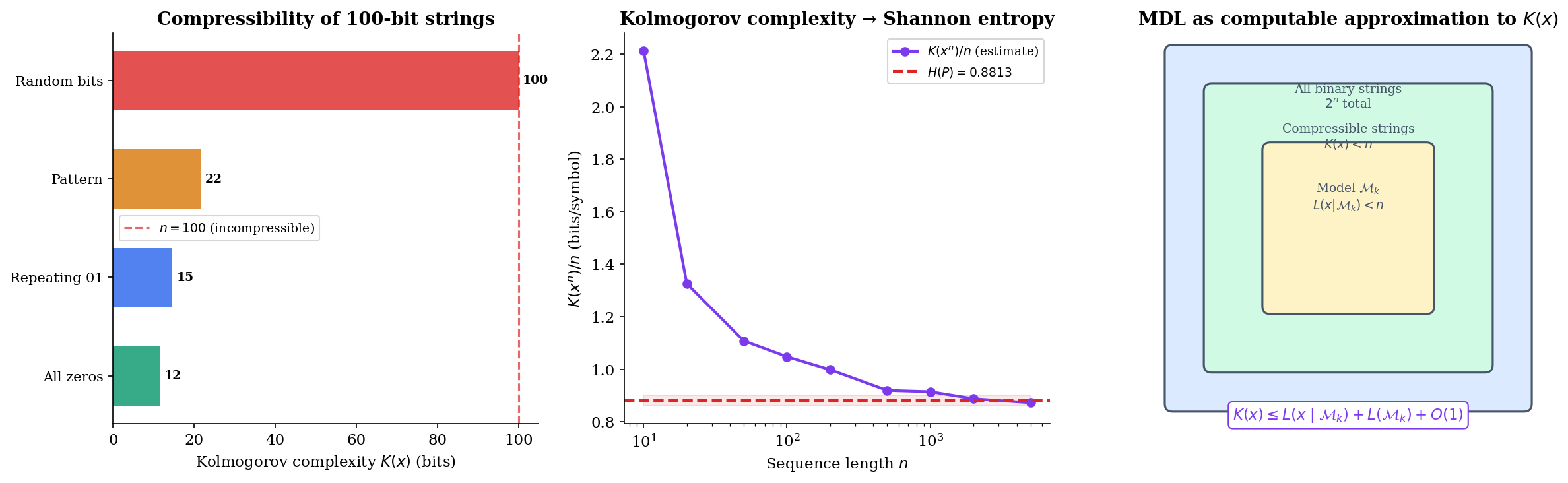
$K(x)$ captures the intuitive notion of the “true complexity” of a string. A string of all zeros has low Kolmogorov complexity (a short loop produces it), while a random string has complexity close to its length (no program shorter than the string itself can produce it).

Theorem 1 (Invariance Theorem).

For any two universal Turing machines $U$ and $V$ , there exists a constant $c_{U,V}$ (depending only on $U$ and $V$ , not on $x$ ) such that:

$|K_U(x) - K_V(x)| \leq c_{U,V}$

for all strings $x$ .

Proof.

The key idea is simulation. Since $V$ is universal, there exists a program $s$ that makes $V$ simulate $U$ . For any string $x$ with $U(p) = x$ , we can construct a program for $V$ : the simulator $s$ followed by $p$ . This gives $K_V(x) \leq |s| + K_U(x)$ . By symmetry, $K_U(x) \leq |s'| + K_V(x)$ for some simulator $s'$ . Setting $c_{U,V} = \max(|s|, |s'|)$ completes the proof.

∎

The invariance theorem means that Kolmogorov complexity is well-defined up to an additive constant — the choice of reference machine doesn’t matter asymptotically. We drop the subscript $U$ and write simply $K(x)$ .

The fundamental connection between Kolmogorov complexity and Shannon entropy:

Proposition 1 (Kolmogorov Complexity and Entropy).

If $X_1, X_2, \ldots$ are i.i.d. draws from a distribution $P$ with entropy $H(P)$ , then:

$\frac{K(X_1 X_2 \cdots X_n)}{n} \to H(P) \quad \text{almost surely as } n \to \infty$

Proof.

The upper bound $K(x^n)/n \leq H(P) + \epsilon$ follows from the asymptotic equipartition property (AEP): with high probability, $x^n$ lies in the typical set, which has $2^{n(H(P) + \epsilon)}$ elements. A program that encodes the index within the typical set uses $n(H(P) + \epsilon)$ bits. The lower bound comes from the incompressibility lemma: random strings cannot be systematically compressed below their entropy rate.

∎

This proposition reveals the deep connection: Kolmogorov complexity is the individual-sequence analogue of Shannon entropy. But there’s a fatal practical problem: $K(x)$ is uncomputable. No algorithm can compute $K(x)$ for all inputs — this follows from the halting problem. MDL sidesteps uncomputability by restricting to computable coding schemes, providing a practical upper bound on $K(x)$ .

Three-panel figure showing string compressibility, K(x^n)/n convergence to entropy, and MDL as a computable approximation

Stochastic Complexity & Refined MDL

Crude MDL has a troubling dependence on arbitrary choices: the precision $b$ used to encode coefficients, the integer code for model indices. Refined MDL eliminates these choices by using a single universal code — the Normalized Maximum Likelihood (NML) distribution.

Definition 4 (Stochastic Complexity).

The stochastic complexity of a data sequence $x^n$ relative to a parametric model class $M_k = \{p_\theta : \theta \in \Theta_k\}$ is:

$\mathrm{SC}(x^n; M_k) = -\log_2 p_{\mathrm{NML}}(x^n \mid M_k)$

where $p_{\mathrm{NML}}$ is the Normalized Maximum Likelihood distribution defined below.

Definition 5 (Normalized Maximum Likelihood (NML)).

The NML distribution for model class $M_k$ is:

$p_{\mathrm{NML}}(x^n \mid M_k) = \frac{p(x^n \mid \hat{\theta}(x^n), M_k)}{\mathrm{COMP}(M_k)}$

where $\hat{\theta}(x^n)$ is the maximum likelihood estimator for data $x^n$ , and the parametric complexity is the normalizing constant:

$\mathrm{COMP}(M_k) = \sum_{z^n \in \mathcal{X}^n} p(z^n \mid \hat{\theta}(z^n), M_k)$

The sum ranges over all possible data sequences of length $n$ . (For continuous data, the sum becomes an integral.)

The NML distribution is remarkable: it assigns to each dataset the maximum likelihood for that dataset, but normalized so the result is a proper probability distribution. Why is this a good universal code?

Theorem 2 (Shtarkov's Minimax Optimality).

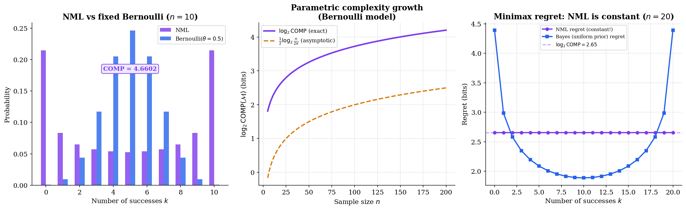
The NML distribution achieves constant regret across all data sequences:

$\log_2 \frac{p(x^n \mid \hat{\theta}(x^n))}{p_{\mathrm{NML}}(x^n)} = \log_2 \mathrm{COMP}(M_k)$

for all $x^n$ . Moreover, NML is the unique distribution achieving the minimax regret:

$p_{\mathrm{NML}} = \arg\min_{q} \max_{x^n} \log_2 \frac{p(x^n \mid \hat{\theta}(x^n))}{q(x^n)}$

Proof.

The regret of NML is:

$\log_2 \frac{p(x^n \mid \hat{\theta}(x^n))}{p_{\mathrm{NML}}(x^n)} = \log_2 \frac{p(x^n \mid \hat{\theta}(x^n)) \cdot \mathrm{COMP}}{p(x^n \mid \hat{\theta}(x^n))} = \log_2 \mathrm{COMP}$

This is constant — it does not depend on $x^n$ . For any other distribution $q$ , the maximum regret over all $x^n$ is at least $\log_2 \mathrm{COMP}$ . To see this, suppose $q$ achieves maximum regret $R^* < \log_2 \mathrm{COMP}$ . Then for all $x^n$ :

$q(x^n) \geq p(x^n \mid \hat{\theta}(x^n)) \cdot 2^{-R^*}$

Summing over all $x^n$ : $1 = \sum_{x^n} q(x^n) \geq 2^{-R^*} \cdot \mathrm{COMP} > 1$ , a contradiction. Therefore NML achieves the minimax regret, and this regret equals $\log_2 \mathrm{COMP}$ .

∎

The interactive visualization below shows NML in action for the Bernoulli model. Notice that the NML regret (purple line) is perfectly flat — constant across all possible numbers of successes. The comparison codes (Bayes, plug-in) achieve lower regret for some outcomes but much higher regret for others.

Sample size n:20Comparison code:

Three-panel figure showing NML vs Bernoulli distributions, parametric complexity growth, and minimax regret

Fisher Information & Asymptotic Complexity

Computing $\mathrm{COMP}$ exactly requires summing over all possible datasets — exponential in $n$ . Rissanen’s asymptotic expansion reveals the geometric structure hiding inside this sum.

Theorem 3 (Asymptotic Parametric Complexity (Rissanen 1996)).

For a $k$ -dimensional parametric model class $M_k$ with parameter space $\Theta_k$ and Fisher information matrix $I(\theta)$ , as $n \to \infty$ :

$\log \mathrm{COMP}(M_k) = \frac{k}{2} \log \frac{n}{2\pi} + \log \int_{\Theta_k} \sqrt{\det I(\theta)} \, d\theta + o(1)$

This expansion has a beautiful geometric interpretation:

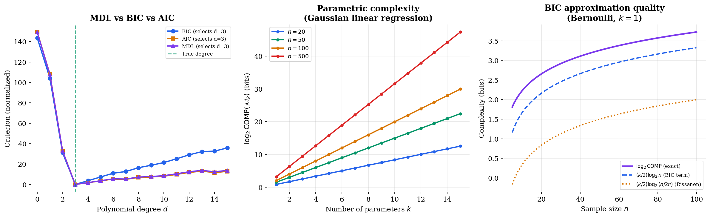
The $\frac{k}{2} \log \frac{n}{2\pi}$ term is the dominant contribution — it grows with both the number of parameters $k$ and the sample size $n$ . This is essentially the BIC penalty.
The integral $\int \sqrt{\det I(\theta)} \, d\theta$ is the volume of the model manifold in the Fisher information metric. Models with larger parameter spaces (in the Fisher metric sense) receive a larger complexity penalty. This is the term that distinguishes refined MDL from BIC.

Corollary 1 (Stochastic Complexity ≈ BIC + Geometry).

The stochastic complexity can be approximated as:

$\mathrm{SC}(x^n; M_k) \approx -\log_2 p(x^n \mid \hat{\theta}) + \frac{k}{2} \log_2 \frac{n}{2\pi} + \log_2 \int_{\Theta_k} \sqrt{\det I(\theta)} \, d\theta$

The first two terms match the BIC (up to additive constants); the third term is the geometric correction that BIC misses.

Proposition 2 (BIC as Crude MDL Approximation).

The Bayesian Information Criterion:

$\mathrm{BIC} = -2 \log L(\hat{\theta}) + k \log n$

is a rough approximation to twice the stochastic complexity, dropping the Fisher information integral and using $\log n$ in place of $\log(n / 2\pi)$ . BIC is consistent (selects the true model as $n \to \infty$ ) but generally less accurate than refined MDL for finite samples.

Remark (BIC as Practical MDL).

When to use BIC vs. refined MDL: BIC is appropriate for quick model comparison when exact Fisher information computation is infeasible, or when the models being compared have the same functional form (the Fisher integral cancels in the difference). Refined MDL (stochastic complexity) is preferable when comparing models of different types — e.g., Gaussian vs. Poisson — where the Fisher volumes differ.

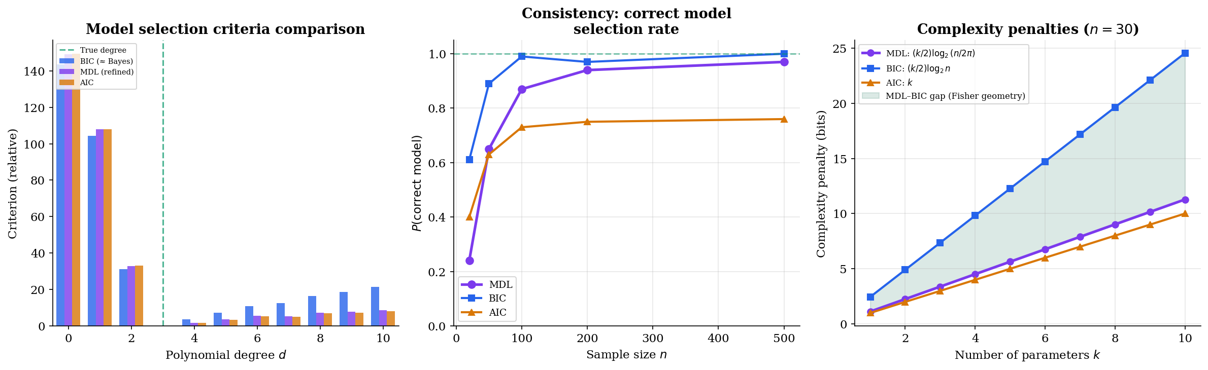
The visualization below compares all three criteria. Note that MDL and BIC agree on the selected model degree most of the time, but AIC tends to overfit — it selects higher-degree models because its penalty ( $2k$ ) doesn’t grow with sample size.

True degree:Noise σ:0.30Display n:100

Three-panel figure showing BIC vs AIC vs MDL, parametric complexity growth, and BIC approximation quality

MDL and Bayesian Model Selection

MDL and Bayesian model selection appear to come from completely different philosophical traditions — coding theory vs. probabilistic inference. Yet they converge asymptotically in a surprising way.

Theorem 4 (Bayesian Marginal Likelihood and Stochastic Complexity).

Under Jeffreys prior $\pi_J(\theta) \propto \sqrt{\det I(\theta)}$ , the log marginal likelihood satisfies:

$-\log \int p(x^n \mid \theta) \pi_J(\theta) \, d\theta = \mathrm{SC}(x^n; M_k) + o(1)$

as $n \to \infty$ . That is, the stochastic complexity and the negative log marginal likelihood under Jeffreys prior are asymptotically equivalent.

Proof.

By Laplace approximation, the marginal likelihood concentrates around the MLE:

$\int p(x^n \mid \theta) \pi_J(\theta) \, d\theta \approx p(x^n \mid \hat{\theta}) \cdot \pi_J(\hat{\theta}) \cdot (2\pi)^{k/2} \cdot |\mathcal{I}_n(\hat{\theta})|^{-1/2}$

where $\mathcal{I}_n(\hat{\theta}) = n \cdot I(\hat{\theta})$ is the observed Fisher information. Taking the negative logarithm:

$-\log \int p(x^n \mid \theta) \pi_J(\theta) \, d\theta \approx -\log p(x^n \mid \hat{\theta}) + \frac{k}{2} \log \frac{n}{2\pi} + \log \frac{\int \sqrt{\det I(\theta)} \, d\theta}{\sqrt{\det I(\hat{\theta})}} + \frac{1}{2} \log \det I(\hat{\theta})$

Collecting terms and using $\pi_J(\hat{\theta}) = \sqrt{\det I(\hat{\theta})} / \int \sqrt{\det I(\theta)} \, d\theta$ , we recover the stochastic complexity up to $o(1)$ terms.

∎

This equivalence explains a deep fact: Jeffreys prior is not just a convenient default — it is the unique prior that makes Bayesian model selection asymptotically equivalent to MDL. Despite their different foundations (MDL is frequentist and prior-free; Bayesian inference requires a prior), the two frameworks agree in the large-sample limit when the Bayesian uses the “right” prior.

The philosophical differences remain important:

MDL treats the code length as fundamental — models are evaluated by their compression efficiency. No prior is needed; the parametric complexity arises from the structure of the model class itself.
Bayesian model selection treats the posterior probability as fundamental — models are evaluated by how well they predicted the data, averaged over the prior. The prior encodes genuine beliefs about which parameter values are more plausible.
When the prior is misspecified (i.e., not Jeffreys), the two methods can disagree — and MDL is often more robust because it doesn’t rely on prior correctness.

Three-panel figure showing MDL vs Bayesian selection, marginal likelihood curves, and model selection agreement

Prequential Codes & Online MDL

There’s a practical problem with NML: computing $\mathrm{COMP}$ requires summing over all possible datasets of length $n$ . For many model classes, this sum is intractable. Prequential (predictive) MDL bypasses this entirely by processing data sequentially.

Definition 6 (Prequential Code).

The prequential code length for a data sequence $x^n = (x_1, x_2, \ldots, x_n)$ under a sequential prediction strategy $q$ is:

$L_{\mathrm{pre}}(x^n) = -\sum_{i=1}^{n} \log_2 q(x_i \mid x^{i-1})$

where $q(x_i \mid x^{i-1})$ is the predictive probability assigned to $x_i$ given the first $i-1$ observations.

The prequential code is always a valid code (Kraft inequality is satisfied by the chain rule of probability), and it’s always computable — no normalization over all possible datasets is needed.

A natural prediction strategy is the prequential plug-in code: use the MLE fitted on past data to predict the next observation. For the Bernoulli model with Laplace smoothing:

$q(x_i \mid x^{i-1}) = \frac{k_{i-1} + 1}{i - 1 + 2} \cdot \mathbf{1}[x_i = 1] + \frac{i - 1 - k_{i-1} + 1}{i - 1 + 2} \cdot \mathbf{1}[x_i = 0]$

where $k_{i-1}$ is the number of ones in the first $i-1$ observations.

Theorem 5 (Prequential Code and Stochastic Complexity).

The prequential plug-in code achieves:

$L_{\mathrm{pre}}(x^n) = \mathrm{SC}(x^n; M_k) + o(\log n)$

as $n \to \infty$ . That is, the prequential code converges to the stochastic complexity, with the same leading-order complexity penalty.

Proposition 3 (Consistency of MDL).

Let $M_1 \subset M_2 \subset \cdots$ be a nested sequence of model classes with $M_{k_0}$ being the smallest class containing the true distribution. Both NML-based and prequential MDL select $M_{k_0}$ with probability tending to 1 as $n \to \infty$ , provided the parametric complexity grows as $\frac{k}{2} \log n + O(1)$ .

Proof.

For any model $M_k$ with $k > k_0$ , the difference in stochastic complexities satisfies:

$\mathrm{SC}(x^n; M_k) - \mathrm{SC}(x^n; M_{k_0}) = \frac{k - k_0}{2} \log n + O(1) - [\log L_k(\hat{\theta}_k) - \log L_{k_0}(\hat{\theta}_{k_0})]$

The log-likelihood difference is $O_P(1)$ (bounded in probability by Wilks’ theorem), while the complexity penalty grows as $\frac{k - k_0}{2} \log n \to \infty$ . Therefore overly complex models are eventually penalized out. For $k < k_0$ , the log-likelihood penalty grows linearly in $n$ (model misspecification), outpacing any complexity savings. The true model minimizes stochastic complexity asymptotically.

∎

Proposition 4 (Prequential Code via Bayes Mixture).

The prequential code using a Bayesian predictive distribution with prior $\pi$ :

$q_\pi(x_i \mid x^{i-1}) = \frac{\int p(x^i \mid \theta) \pi(\theta) \, d\theta}{\int p(x^{i-1} \mid \theta) \pi(\theta) \, d\theta}$

yields a prequential code length equal to the negative log marginal likelihood:

$L_{\mathrm{pre}}(x^n) = -\log_2 \int p(x^n \mid \theta) \pi(\theta) \, d\theta$

This is a consequence of the chain rule: $p(x^n) = \prod_{i=1}^{n} p(x_i \mid x^{i-1})$ .

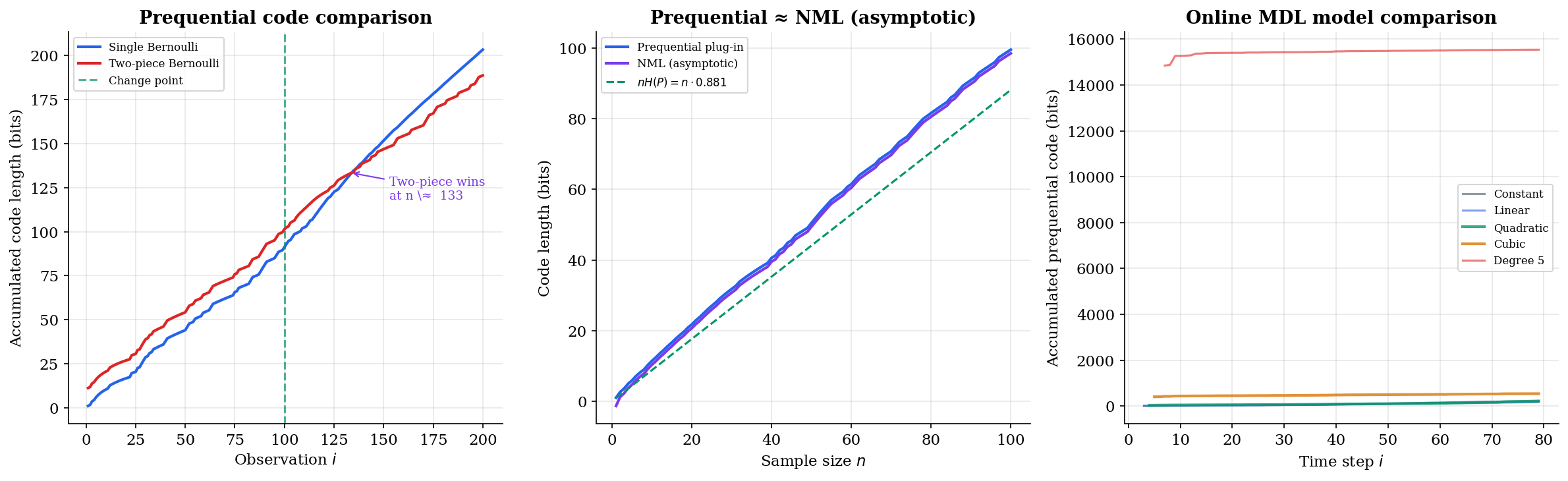
The visualization below shows prequential MDL in action for change-point detection. Two models compete: a single Bernoulli (one parameter for the whole sequence) and a two-piece Bernoulli (different parameters before and after a change point). Watch how the two-piece model initially incurs higher overhead but eventually wins when the distributional shift becomes evident.

Scenario:Change at:50%p₁:0.30p₂:0.70

i = 0 / 200

Three-panel figure showing prequential code comparison, online model selection, and sequential adaptation

MDL for Practical Model Selection

How does MDL translate to the everyday tasks of machine learning: choosing features, selecting the number of components, detecting overfitting?

Proposition 5 (MDL for Linear Regression).

For linear regression with $k$ features, $n$ observations, and Gaussian errors, the refined MDL criterion reduces to:

$\mathrm{MDL}(M_k) = \frac{n}{2} \log(2\pi e \hat{\sigma}_k^2) + \frac{k}{2} \log \frac{n}{2\pi} + c_k$

where $\hat{\sigma}_k^2 = \text{RSS}_k / n$ and $c_k$ depends on the Fisher information geometry. When $c_k$ is ignored (equal across models), this reduces to BIC up to a constant.

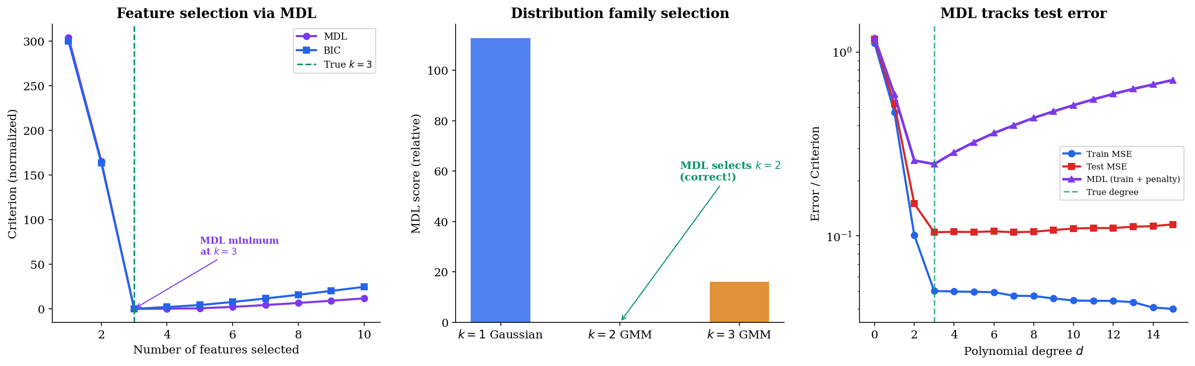
Feature selection via MDL. In forward feature selection, we greedily add the feature that reduces the total MDL criterion the most. The MDL penalty automatically trades off the improvement in fit against the cost of an additional parameter. Unlike cross-validation, MDL requires no held-out data.

Theorem 6 (MDL Consistent Model Selection).

Let the true model have $k_0$ nonzero features. Forward selection using the MDL (or BIC) criterion selects $k_0$ features with probability tending to 1 as $n \to \infty$ , provided:

The penalty grows as $\frac{k}{2} \log n$ (satisfied by both BIC and MDL).
The penalty grows slower than $n$ (ensuring we don’t underfit).

AIC is not consistent: its fixed penalty $2k$ allows overfitting to persist even as $n \to \infty$ .

Proof.

The proof follows the same logic as Proposition 3. For any model with $k > k_0$ features, the likelihood improvement from the $k - k_0$ spurious features is $O_P(\chi^2_{k-k_0})$ (by Wilks’ theorem), while the penalty cost is $\frac{k-k_0}{2} \log n \to \infty$ . So spurious features are eventually rejected. For AIC, the penalty is $k - k_0$ (constant), which does not dominate the $O_P(1)$ likelihood improvement, so AIC selects too many features with non-vanishing probability.

∎

Three-panel figure showing MDL feature selection, distribution family selection, and MDL tracking test error

Computational Notes

MDL in Practice: BIC as a Proxy

For most practical applications, BIC is a reasonable proxy for MDL:

$\mathrm{BIC} = -2 \log L(\hat{\theta}) + k \log n$

BIC is fast to compute, consistent, and readily available in every statistics package. Use it when:

Comparing models of the same type (the Fisher volume term cancels)
The sample size $n$ is large enough that asymptotic approximations hold
You don’t need the geometric correction from the Fisher information

Remark (MDL and Regularization).

The MDL penalty on model complexity has a natural connection to $L_0$ regularization — penalizing the number of nonzero parameters. The refined MDL score $-\log L(\hat{\theta}) + \frac{k}{2} \log n$ assigns a cost of roughly $\frac{1}{2} \log n$ bits per parameter. In the regression setting, this is equivalent to an $L_0$ penalty with strength $\lambda = \frac{1}{2} \log n$ . Unlike $L_1$ or $L_2$ regularization (which shrink parameters toward zero), the MDL/ $L_0$ approach performs hard selection: each feature is either in the model or out.

Remark (MDL and Neural Network Compression).

MDL provides an information-theoretic framework for understanding neural network compression. The total description length of a network is $L(\text{architecture}) + L(\text{weights} \mid \text{architecture}) + L(\text{data} \mid \text{network})$ . Pruning (removing weights), quantization (reducing precision), and knowledge distillation (compressing into a smaller network) can all be understood as reducing the first two terms. The lottery ticket hypothesis — that sparse subnetworks can match the performance of the full network — is a statement about MDL: the compressed description (sparse architecture + remaining weights) has lower total code length than the full network. This connects modern deep learning compression to Rissanen’s 1978 insight that the best model is the one with the shortest total description.

Summary Comparison

Criterion	Formula	Penalty	Consistent?	Requires
AIC	$-2 \log L + 2k$	Fixed ( $2k$ )	No	Only $\hat{\theta}$ , $k$
BIC	$-2 \log L + k \log n$	$O(\log n)$	Yes	Only $\hat{\theta}$ , $k$ , $n$
Refined MDL	$-2\log L + k\log\frac{n}{2\pi} + 2\log \int\sqrt{\det I(\theta)} \, d\theta$	$O(\log n) +$ geometry	Yes	Fisher information
NML (exact)	$-\log p_{\mathrm{NML}}$	Minimax optimal	Yes	COMP enumeration
Prequential MDL	$-\sum \log q(x_i \mid x^{i-1})$	Adaptive	Yes	Sequential predictions

Connections & Further Reading

Connection Map

Topic	Relationship
Shannon Entropy & Mutual Information	MDL formalizes source coding for model selection: the shortest description length equals the entropy $H(P)$ under the true model. Shannon’s source coding theorem underpins the coding interpretation of MDL.
KL Divergence & f-Divergences	The regret of a universal code is bounded by $D_{\mathrm{KL}}(p_{\theta^*} \\| p_{\mathrm{NML}})$ . The stochastic complexity decomposes into the maximized log-likelihood plus the KL divergence from the NML distribution to the MLE model.
Rate-Distortion Theory	Rate-distortion theory and MDL are dual perspectives on compression: rate-distortion minimizes bits for a fidelity constraint, while MDL uses total description length for model selection. The information bottleneck connects both viewpoints.
Convex Analysis	The NML optimization is a minimax problem solved by convex duality. The parametric complexity integral involves the Fisher information geometry, connecting to the convex structure of exponential families.
Information Geometry & Fisher Metric	The asymptotic parametric complexity $\log \mathrm{COMP}$ involves $\int \sqrt{\det I(\theta)} \, d\theta$ — the volume of the model manifold in the Fisher metric. MDL model complexity has a geometric interpretation as the “size” of the model in information space.
PAC Learning & Computational Learning Theory (coming soon)	MDL and PAC learning provide complementary perspectives on generalization: MDL penalizes model complexity via description length, while PAC bounds generalization error via VC dimension. Occam’s razor lemma connects both: short descriptions imply small generalization error.

Notation Reference

Symbol	Meaning
$L(M)$	Code length for model $M$ (complexity)
$L(D \mid M)$	Code length for data $D$ given model $M$ (goodness-of-fit)
$L^*(k)$	Rissanen’s universal code for positive integer $k$
$K(x)$	Kolmogorov complexity of string $x$
$\mathrm{SC}(x^n; M_k)$	Stochastic complexity of $x^n$ under model $M_k$
$p_{\mathrm{NML}}$	Normalized Maximum Likelihood distribution
$\mathrm{COMP}(M_k)$	Parametric complexity: $\sum_{z^n} p(z^n \mid \hat{\theta}(z^n))$
$I(\theta)$	Fisher information matrix at parameter $\theta$
$\hat{\theta}(x^n)$	Maximum likelihood estimator for data $x^n$
$L_{\mathrm{pre}}(x^n)$	Prequential (predictive) code length
$\mathrm{BIC}$	Bayesian Information Criterion: $-2 \log L + k \log n$

Overview & Motivation

What We Cover

Two-Part Codes & Crude MDL

Encoding Models

Example: Polynomial Regression

Kolmogorov Complexity

Stochastic Complexity & Refined MDL

Fisher Information & Asymptotic Complexity

MDL and Bayesian Model Selection

Prequential Codes & Online MDL

MDL for Practical Model Selection

Computational Notes

MDL in Practice: BIC as a Proxy

Summary Comparison

Connections & Further Reading

Connection Map

Notation Reference

Connections

References & Further Reading